
A maintenance team usually knows the feeling before the data confirms it. A pump trips again on second shift. A gearbox work order gets closed with a vague note like “repaired and returned to service.” The weekly review says reliability is slipping, but nobody agrees on how often the asset fails, what counts as a failure, or whether the run-time data in the CMMS can be trusted.
That's where teams need discipline, not another dashboard. To calculate mean time between failure correctly, the arithmetic is simple. The hard part is deciding what to count, pulling clean uptime from messy records, and then turning one reliability number into a maintenance decision that changes plant behavior. On the floor, that means knowing whether to tighten a PM interval, launch a root cause investigation, or stop using average-based logic and move to a different analysis method.
Table of Contents
- Defining Failure MTBF vs MTTF and Why It Matters
- Your Calculation Is Only as Good as Your Data
- Calculating Basic MTBF for Industrial Assets
- Moving Beyond Averages with Confidence Intervals
- Common MTBF Calculation Mistakes and How to Avoid Them
- From Calculation to Action Using MTBF in RCM and PM Optimization
Defining Failure MTBF vs MTTF and Why It Matters
A reactor circulation pump trips at 2:13 a.m., production slows, and three people start arguing about the event before the work order is even written. Operations calls it a failure. Maintenance calls it a seal issue that never fully stopped the pump. Stores wants to know whether to stock another repair kit or replace the whole assembly next outage. That disagreement is exactly why MTBF and MTTF need clean definitions before anyone starts calculating anything.
MTBF applies to assets that return to service after repair. MTTF applies to items whose service life ends when they fail and are then replaced. The math is only part of the distinction. The bigger issue on the plant floor is decision quality. Using MTBF for a disposable component, or MTTF for a repairable machine, distorts spares strategy, PM intervals, and lifecycle cost discussions.
For repairable assets, MTBF is typically expressed as total operating time divided by the number of functional failures over that period. MTTF tracks the average operating life to failure for non-repairable items. In practice, the question is less about formula selection and more about how the equipment is maintained in the field. A pump, motor, or gearbox usually belongs in MTBF analysis because the asset is restored and sent back into duty. A fuse, sacrificial sensor, or single-use component usually belongs in MTTF analysis because replacement ends that item's life history.
What counts as a failure
Failure has to mean loss of required function. Without that rule, teams contaminate the count with inspections, cosmetic defects, nuisance alarms, and operator complaints that never affected output, quality, or safe operation.
On a process pump, a failure might mean loss of flow, inability to hold pressure, repeated trips, or a condition that required corrective work to keep the asset running within operating limits. A minor oil seep that needs monitoring but does not affect duty is a defect. It may matter for planning, but it should not automatically be counted as a failure event in MTBF.
That distinction sounds academic until two sites compare numbers. One site logs every seal leak as a failure. Another only logs a failure when the pump can no longer meet process demand. Both sites can produce an MTBF value. Only one is likely to support a useful maintenance decision.
Practical rule: Count events that required corrective action to restore required function. Track developing defects separately so they do not inflate failure frequency.
Why teams mix up MTBF and MTTF
The confusion usually starts in CMMS coding and spare parts habits, not in reliability theory. A repairable motor may be replaced at the asset level, then sent to the shop for rebuild. The storeroom sees a replacement. Reliability sees a repairable population. If the work order structure does not separate those actions, the wrong metric gets attached to the equipment class.
Here is the clean split:
| Metric | Best used for | Typical examples |
|---|---|---|
| MTBF | Repairable assets | motors, compressors, pumps, gearboxes |
| MTTF | Non-repairable items | fuses, some electronic boards, single-use components |
Mixing terms leads to hidden costs later. Teams set PM frequencies off an average that does not match the asset's failure behavior. They over-maintain equipment that fails randomly, or they miss age-related wear because they never separated repairable assemblies from consumable parts. That is one reason reliability teams should understand equipment failure patterns and the six curves of maintenance before turning an average life number into a maintenance task.
Operational time means actual time under duty
MTBF is based on operating exposure, not just elapsed calendar time. A standby fire pump, a batch mixer, and a continuously loaded compressor accumulate stress in very different ways. Treating all three as though they age on the same clock produces clean-looking numbers that are still wrong.
Use runtime that matches the duty being analyzed. For rotating equipment, that usually means actual running hours, or loaded hours if load swings materially affect degradation. Pair that time basis with the same failure definition every time. Once those two pieces are stable, MTBF becomes useful for more than reporting. It becomes a decision input for PM, condition monitoring, and RCM work.
Your Calculation Is Only as Good as Your Data
A maintenance team can spend an afternoon building an MTBF report, get a clean number to two decimal places, and still be wrong by a wide margin. The failure is usually upstream. Bad closeout discipline, missing runtime, and loose failure coding distort the result long before anyone touches the formula.
On the plant floor, this shows up in familiar ways. A packaging conveyor jams six times a shift, but only the long stoppages become work orders. A standby pump gets credited with calendar hours instead of run hours. A compressor trip creates three separate records from operations, maintenance, and planning, and all three get counted as failures. The final MTBF looks precise, but it is built on mixed definitions and partial history.

What clean MTBF data requires
Good MTBF data has three things in place. A clear failure definition. A defensible measure of operating exposure. A work order history that ties each failure event to the right asset and the right time period.
That sounds simple until the CMMS meets real operating conditions. Plants run partial shifts. Loads change by season or product mix. Equipment cycles between running, idle, and standby. If those states are not separated in the source data, uptime gets overstated and the average life between failures looks better than reality.
The practical fix is consistency, not perfection. Pick one asset class, define failure in language supervisors and technicians both use, then test the report against known events from the last few months.
A CMMS data quality audit that helps
Start with one problem asset. A pump with repeated seal work, a conveyor with nuisance stops, or a blower everyone complains about is usually enough to expose the weak points in the data.
Check the history in this order:
- Confirm the asset boundary: Keep the record tied to the same physical scope every time. Do not mix a motor-only history with the full pump train or skid.
- Review failure coding: Separate breakdowns from inspections, PM work, operator calls, and planned outage tasks.
- Check timestamp quality: Start and finish times should exist, follow sequence, and reflect the event that happened. Default values and after-the-fact entries skew uptime fast.
- Separate operating states: Running, idle, standby, and planned shutdown need their own logic in the query.
- Read technician comments: Many plants record the useful detail in the notes while the coded failure field stays vague.
- Remove duplicate event records: One functional failure can create several work orders. Count the event once.
- Compare against operator logs: Short recurring stops often never reach maintenance history, especially on packaging and converting lines.
A CMMS preserves plant discipline. It does not create it.
Role clarity matters here. Operators should record when function was lost. Technicians should document what failed and what restored function. Planners should enforce closeout rules. Reliability engineers should review coding logic and test report output against known bad days, not just trust the dashboard. Teams that need to tighten those basics often benefit from a structured CMMS implementation guide for maintenance teams.
What usually goes wrong
Three mistakes show up repeatedly.
Teams use calendar hours because they are easy to export. That inflates MTBF for standby and lightly loaded assets.
Failure codes drift over time. “Repair,” “breakdown,” “follow-up,” and “operator issue” end up lumped together, so nobody can tell what should count in the denominator.
Microstops get ignored. On high-speed lines, those short events are often the first sign that reliability is slipping. Leave them out, and the MTBF number stops being useful for PM review, condition-based monitoring thresholds, or RCM decisions.
The point is not to create perfect data before doing any analysis. The point is to get the data clean enough that the final MTBF supports a real maintenance decision instead of giving false confidence.
Calculating Basic MTBF for Industrial Assets
A maintenance planner pulls a year of compressor history, divides hours by failures, and gets a clean MTBF number. Then the team uses it to stretch a PM interval and gets burned two months later. The math was fine. The event selection was not.
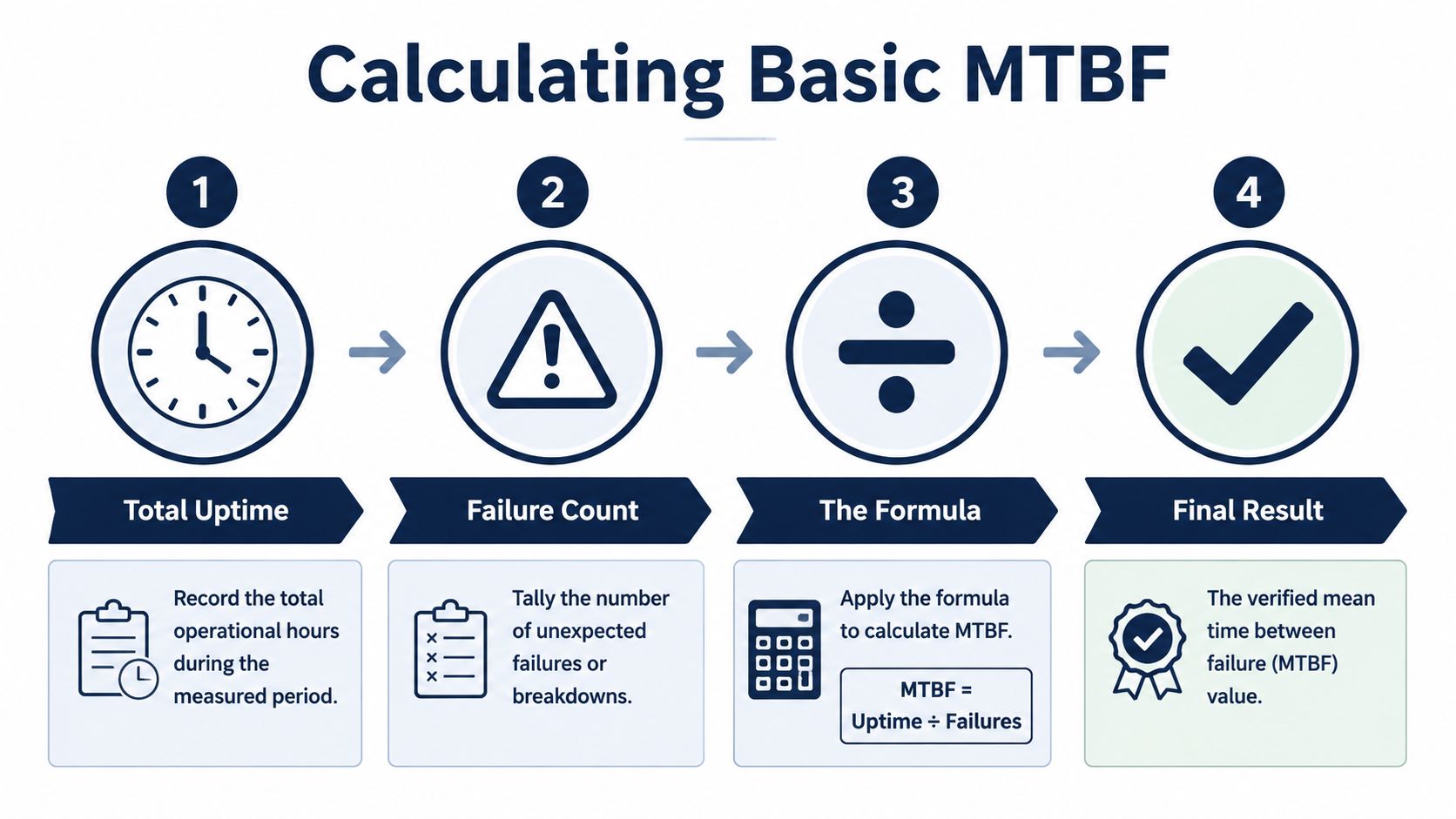
For a repairable asset, the basic calculation is still simple:
Formula: MTBF = Total Operating Time ÷ Number of Failures
The hard part is deciding what belongs in each side of that equation. In plant work, that means matching counted failures to the same operating window that produced the runtime. If the numerator comes from meter hours but the denominator includes every corrective work order in the CMMS, the result is distorted before anyone opens a spreadsheet.
A refinery compressor example
Use a centrifugal compressor with one year of history. Start by fixing the study boundary before doing any arithmetic. Define the asset tag, the date range, the operating state that counts as uptime, and the failure definition tied to lost function.
Then review the work history. Remove PM tasks, inspections, deferred defects, planned outage work, and follow-up jobs that did not represent a new failure event. Keep only the corrective events that required action to restore the compressor's intended function.
A practical workflow looks like this:
| Step | What the team does | Common trap |
|---|---|---|
| Collect runtime | Pull meter or run-state hours for the exact study period | Using calendar hours or nameplate assumptions |
| Screen failures | Count only corrective events tied to functional loss | Counting every work order as a failure |
| Align timestamps | Make sure each failure occurred within the same operating window | Mixing periods, shifts, or asset states |
| Calculate MTBF | Divide operating time by counted failures | Skipping the assumption log |
Suppose the compressor accumulated 6,000 true operating hours during the review period and had 5 counted failures. Basic MTBF is 1,200 operating hours. That result is useful because the team can now compare it against the current PM interval, the asset's criticality, and the consequences of an in-service trip.
That last step matters more than the arithmetic. A 1,200-hour MTBF does not automatically mean a PM should be set at 1,000 hours. If failures are random, a shorter PM may add cost without reducing risk. If the dominant mode is wear-related and the repair history shows a consistent pattern, a time-based task may make sense. MTBF is an input to the maintenance decision, not the decision itself.
Handling partially observed intervals
Assets rarely fail on a neat schedule that matches the reporting window. A pump may run for months after its last recorded failure, and the study period can end before the next one occurs. That operating time still belongs in the analysis if the team's method includes all observed uptime within the window.
The key is consistency. Use the same treatment for every asset in the population and document it. If one monthly report includes trailing uptime after the last failure and the next report excludes it, trend charts stop reflecting asset behavior and start reflecting reporting choices.
I tell new engineers to write the rule down before they run the report. If the rule lives only in the analyst's head, the metric will drift as soon as someone else inherits the workbook.
Quick checks before you trust the result
A few basic checks catch many bad MTBF calculations:
- Failure count of zero with a reported MTBF value. That should usually be shown as insufficient failure data or handled by a defined reporting rule.
- Operating hours that exceed what the asset could physically accumulate in the study period.
- Failure events clustered around a shutdown that were one underlying defect.
- Fleet averages built from assets with very different duty cycles, loads, or environments.
These checks save rework. They also prevent a bad MTBF from driving the wrong action, such as adding PM labor to a random failure mode or missing an obvious candidate for condition monitoring.
For teams that want to place MTBF alongside the other operating metrics used in reliability reviews, this guide to MTBF, MTTR, and OEE in reliability metrics gives the broader context.
Moving Beyond Averages with Confidence Intervals
A single MTBF number looks authoritative, but it can hide a lot of uncertainty. That's especially true when the team is working with a small number of failures, a short study window, or assets that operate in varying duty conditions. A boiler feed water pump with a handful of breakdowns can produce an average that appears stable while the underlying uncertainty is still wide.
That's where confidence intervals help. They don't replace MTBF. They add context around how much trust the team should place in the estimate before changing PM strategy, buying spares, or escalating to a capital project.

What the range means in practice
A narrow interval tells a maintenance manager that the observed failure history is reasonably stable under the conditions studied. A wide interval says something different. The asset may still be poorly understood, the sample size may be small, or the operating context may be too mixed for one average to carry much decision weight.
For a power generation site, that matters. If a feed pump's estimated MTBF is based on sparse events, a major PM rescheduling decision should be treated cautiously. A weak estimate can push the plant toward over-maintenance or under-maintenance, and both are expensive in different ways.
How engineers use confidence without overcomplicating it
Most plant teams don't need to derive the full statistics by hand every time. What they need is a repeatable method and disciplined interpretation. A reliability engineer can use a standard statistical calculator or internal analysis sheet to estimate a confidence interval for the observed MTBF, then compare that range with the maintenance action under consideration.
Use confidence intervals this way:
- When failures are few: Treat the average as provisional. Don't redesign the PM program around a thin dataset.
- When the range is wide: Break the population apart by duty cycle, asset model, or failure mode before drawing conclusions.
- When the range tightens over time: Confidence improves as the dataset becomes more representative of actual operating conditions.
Averages answer “what was observed.” Confidence intervals help answer “how strongly should the plant act on it.”
Where confidence changes the maintenance decision
Consider a fleet of similar pumps. If one unit shows a deteriorating average but the confidence range is still broad, the plant should first check data quality, operating conditions, and failure mode separation. If the interval is relatively tight and trending downward, that's a stronger trigger for intervention.
The intervention itself should still fit the failure behavior. If the issue is random seal leakage, the answer may be condition-based monitoring and installation review. If the issue is age-related bearing wear, the answer may be interval optimization or deeper life modeling. Confidence intervals don't make the decision. They keep teams from acting too aggressively on unstable evidence.
Common MTBF Calculation Mistakes and How to Avoid Them
Most bad MTBF reports look clean in a meeting. The spreadsheet balances. The chart trends upward or downward. The problem shows up later, when the maintenance plan built on that number doesn't match what the equipment is doing.
An automotive assembly plant offers a familiar example. A fleet of robotic welders may show one blended MTBF value for the entire line, but that average can hide very different behaviors. Mechanical arm wear, cable fatigue, servo faults, and gun-related process interruptions don't belong in one undifferentiated failure bucket if the team is trying to detect an emerging wear-out pattern.

The rogues' gallery of bad MTBF practice
Using calendar time instead of runtime
This is the fastest way to overstate reliability on intermittent assets. The correction is to use actual operating hours tied to the asset state being analyzed.Counting planned work as failure
PM shutdowns, inspections, and scheduled replacements are maintenance activity, not evidence of random failure. Count only events that meet the plant's failure definition.Lumping failure modes together
Bearing wear, lubrication starvation, motor winding faults, and coupling misalignment may all stop the same machine, but they don't mean the same thing analytically. Separate them when making maintenance decisions.Comparing unlike assets
Two pumps with different fluids, loads, speeds, or duty cycles shouldn't be pooled casually. Similar nameplates don't guarantee similar reliability behavior.Ignoring data gaps
Missing timestamps and vague closeout notes are not minor paperwork issues. They directly corrupt the calculation.
Symptom, root cause, correction
| Symptom | Likely root cause | Better approach |
|---|---|---|
| MTBF looks unusually high | Standby or idle time included as uptime | Use actual run hours only |
| MTBF swings sharply month to month | Too few events or inconsistent coding | extend period or improve classification |
| PM interval misses repeat failures | Failure modes blended into one average | calculate by failure mode |
| Fleet average hides a bad actor | Dissimilar assets pooled together | segment by class and duty |
When MTBF is the wrong tool
Some components don't belong in a simple MTBF framework at all. If a part follows a clear wear-out pattern, the plant may need Weibull analysis or another life-distribution approach instead of relying on a single arithmetic average. Teams that keep forcing every problem into MTBF usually end up either changing parts too early or too late.
When the question is “how long until this wear mechanism reaches an unacceptable risk level,” a plain average may be too blunt.
If recurring failures continue after PM changes, the plant should stop recalculating the same metric and investigate causes. A structured root cause analysis process for equipment failures is usually the better next step.
From Calculation to Action Using MTBF in RCM and PM Optimization
A team pulls the monthly reliability report, sees an MTBF improvement, and assumes the maintenance program is working. Then the same line trips twice the next week because the average hid the actual problem. That happens all the time in plants with messy CMMS history and mixed failure coding.
MTBF earns its keep only when it changes a decision. It should affect PM intervals, inspection content, spare holdings, condition monitoring coverage, and the point where the team stops adjusting tasks and starts asking whether the asset needs redesign or a root cause review.
In an RCM program, MTBF is one input, not the conclusion. A shorter interval between failures raises specific questions. Which failure mode is driving the result? Is the failure age-related, random, or induced by operation? Can the mode be detected early enough for a condition-based task to work? Teams building that logic into their asset strategy can use this reliability-centered maintenance implementation guide to connect failure history with task selection.
How MTBF should change the maintenance strategy
The number matters less than the action it supports.
- Stable but low MTBF: Review whether the current PM task addresses the failure mode. If it does, shorten the interval carefully. If it does not, a shorter interval just adds labor without reducing failures.
- Declining MTBF trend: Start a focused failure mode review. Waiting for another quarter of bad history usually means more secondary damage and more unplanned overtime.
- Acceptable asset MTBF but poor line performance: Check the system, controls, utilities, and operating context. The asset may be healthy while the process train remains unreliable.
- No clear trend because records are thin or inconsistent: Fix event quality before changing the maintenance plan. Bad inputs create confident but expensive decisions.
That last case wastes a lot of effort. Plants often change PM frequency when the actual problem is incomplete closeout notes, merged failure codes, or uptime that includes idle hours.
Why the system view changes the answer
A motor, gearbox, and pump can each look acceptable on their own and still produce poor line reliability as a train. For equipment arranged in series, the system fails when any required element fails, so the effective MTBF drops below the standalone MTBF of each component. For a simple series model, system MTBF is calculated as 1 / (1/MTBF_pump + 1/MTBF_gearbox + 1/MTBF_motor). Ignoring that interaction is a common mistake because 40% of industrial downtime stems from interdependent failures (https://www.ibm.com/think/topics/mtbf).
Use a real plant example. A pump train may show repeated pump-end vibration, but the pump is not always the starting point. Soft foot at the motor can drive coupling misalignment, which loads the gearbox and shows up later as seal and bearing failures downstream. If the team only tracks component averages, it keeps replacing parts and misses the mechanism linking the failures.
The same source notes that integrating MTBF analysis with predictive tools such as vibration analysis can extend effective equipment life by 2-3x (https://www.ibm.com/think/topics/mtbf). In practice, that does not mean every asset needs full condition monitoring. It means assets with costly functional failures, weak age-based patterns, or repeated induced failures often need CBM support instead of another calendar-based PM revision.
Where PM, CBM, and RCFA fit
A practical sequence looks like this:
- Calculate MTBF using clean run-time and failure definitions.
- Break the history down by failure mode where the record quality supports it.
- Trend the result over time and compare it with maintenance changes, operating shifts, and process conditions.
- Choose the response that matches the pattern.
If failures show an age-related pattern and the task is technically effective, adjust the PM interval. If failures are random but there is measurable degradation before loss of function, use CBM. If the same failure keeps returning after task changes, launch RCFA instead of recalculating the same average again.
That is the point many teams miss. MTBF is not the strategy. MTBF is a screening metric that helps the team decide whether to prevent, detect, redesign, or investigate.
A plant that can calculate mean time between failure accurately already has an advantage. The bigger payoff comes from turning that number into a specific maintenance decision tied to failure mode, asset criticality, and the quality of the CMMS record.