A vibration alarm during a turnaround week rarely arrives at a convenient time. On a 1,500 kW induced-draft fan, the alert traced back to BPFO harmonics that had climbed over four weekly routes, giving the reliability team enough warning to inspect the bearing before seizure. That is the practical value of bearing defect frequencies. They turn a broad vibration symptom into a focused question about which bearing component is being struck, how the pattern is changing, and whether the maintenance plan needs to move.
Bearing defect frequencies aren't failure thresholds. They're diagnostic fingerprints calculated from bearing geometry and shaft speed. Used correctly, they help maintenance teams distinguish an outer-race defect from an inner-race defect, rolling-element damage, cage wear, lubrication trouble, or unrelated machine vibration. Used carelessly, a single peak near a calculated line can trigger an unnecessary replacement.
Table of Contents
- What Bearing Defect Frequencies Reveal About Machine Health
- Formulas and a Worked Example for the Four Bearing Frequencies
- Matching BPFO BPFI BSF and FTF to Specific Fault Locations
- Why Approximate Frequencies Drift From Real Spectra
- Sampling Rates and Spectrum Settings That Make Defect Frequencies Visible
- Using Envelope Analysis to Surface Hidden Bearing Impacts
- Tracking Defect Frequencies Across Variable Speed Assets
- Common Diagnostic Pitfalls When Reading Bearing Spectra
- Pump Bearing Case Study From First Alert to Replacement
- Field Diagnostic Checklist for Reliability Teams
What Bearing Defect Frequencies Reveal About Machine Health
On route data, a calculated bearing line rarely appears as a single, perfectly placed peak. The analyst may see a weak component in the expected band, several harmonics, or a pattern that shifts with running speed. That distinction matters on plant equipment, where load, slip, structural resonance, lubrication, and sensor location can shape the spectrum as much as the defect itself.
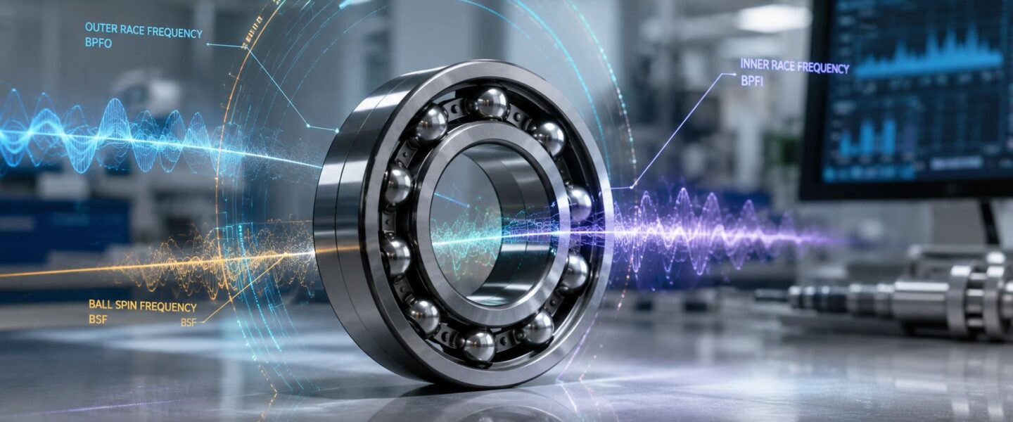
The four diagnostic frequencies identify the bearing component under suspicion:
- FTF, or Fundamental Train Frequency: The cage or retainer rotation rate. Activity here can support a diagnosis involving cage wear, cage damage, or lubrication starvation.
- BPFO, or Ball Pass Frequency Outer: The rate at which rolling elements pass a damaged point on the stationary outer race.
- BPFI, or Ball Pass Frequency Inner: The rate at which rolling elements pass a defect on the rotating inner race.
- BSF, or Ball Spin Frequency: The rotation rate of a ball or roller around its own axis, used when the rolling element itself is damaged.
A route spectrum can therefore narrow the inspection area, but it does not identify repair priority by itself. A peak near BPFO may reflect an outer-race defect, a structural response, or an inaccurate speed and geometry input. The analyst must check whether the component repeats at the expected order, whether its amplitude changes with load, and whether the time waveform contains periodic impacts.
Harmonics and sidebands are most useful when read as a pattern. Harmonics are integer multiples of the calculated defect frequency. Sidebands sit beside a main component and often reflect modulation by shaft speed or cage frequency. A strong harmonic family can make a weak fundamental meaningful, while sideband spacing may indicate how the defect is being loaded during each revolution. Georgia Tech's bearing-fault material describes the four frequencies as indicators for condition monitoring on motor and gearbox bearings.
Practical rule: Use a defect frequency to choose where to investigate. Use amplitude, harmonics, sidebands, trend behavior, operating condition, and inspection evidence to decide what action is justified.
For variable-speed assets, compare orders or resample the data rather than treating a fixed hertz value as permanent. Envelope demodulation can expose repeated impacts hidden beneath running-speed vibration, but resonance and poor measurement settings can still distort the result. Calculated frequencies guide the search. Measurement quality and machine context determine whether the diagnosis holds.
Formulas and a Worked Example for the Four Bearing Frequencies
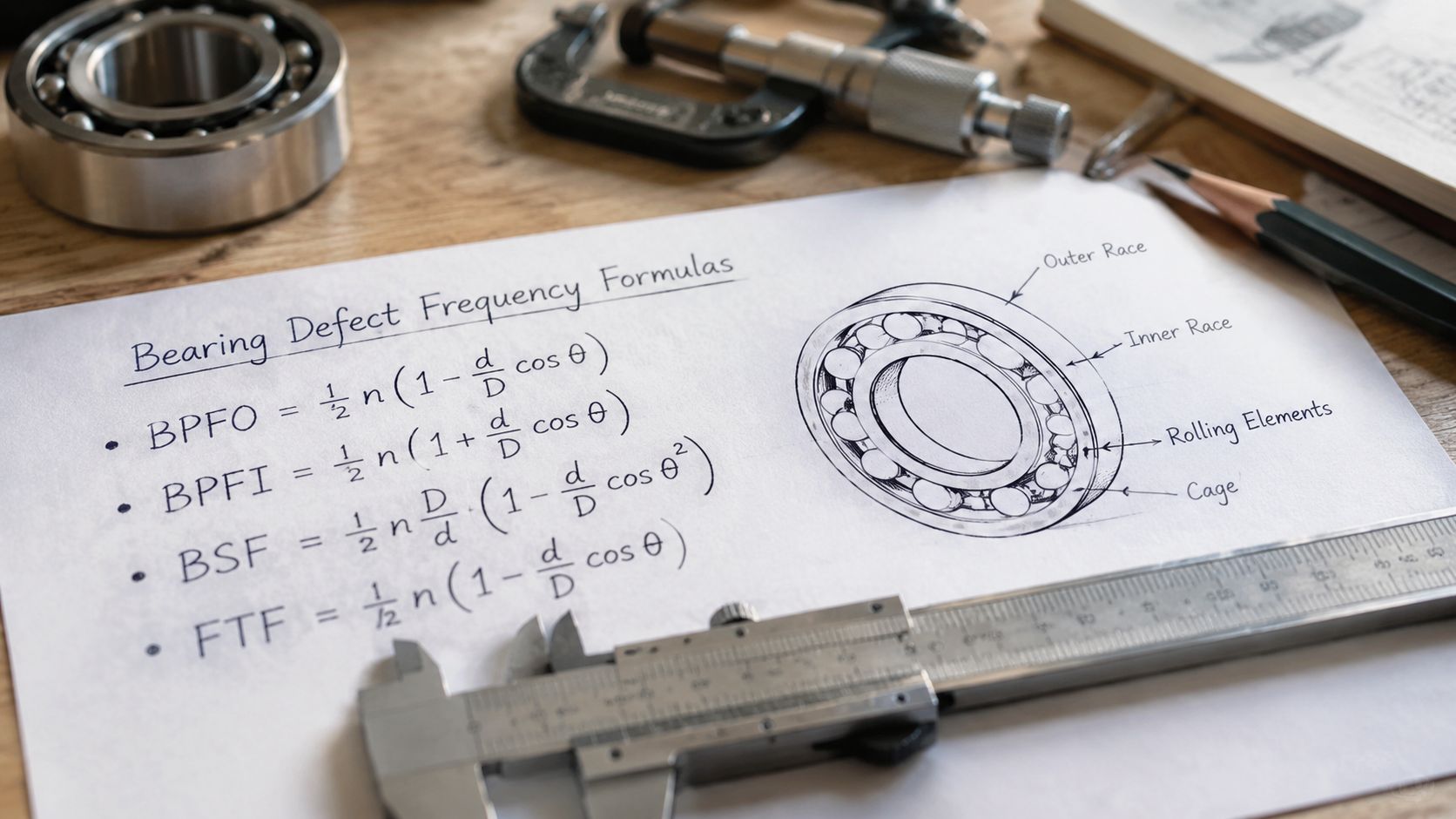
Start with the bearing geometry, then convert shaft speed to frequency. The standard relationships use N for the number of rolling elements, Bd for ball or roller diameter, Pd for pitch diameter, ϕ for contact angle, and fr for shaft frequency:
- BPFO = (N/2) × (1 − Bd/Pd × cos ϕ) × fr
- BPFI = (N/2) × (1 + Bd/Pd × cos ϕ) × fr
- BSF = (Pd/2Bd) × (1 − (Bd/Pd × cos ϕ)²) × fr
- FTF = (1/2) × (1 − Bd/Pd × cos ϕ) × fr
For a 6309-style bearing with 8 rolling elements, Bd/Pd ≈ 0.27, a contact angle of approximately 0°, and a shaft speed of 1,800 RPM:
fr = 1,800 ÷ 60 = 30 Hz
Substituting those values gives four initial search markers:
- BPFO ≈ 104.4 Hz
- BPFI ≈ 135.6 Hz
- BSF ≈ 68.1 Hz
- FTF ≈ 13.05 Hz
The arithmetic also gives a useful check. BPFO + BPFI ≈ N × fr, so the two pass frequencies should total close to 8 × 30 Hz, or 240 Hz. That check can catch an incorrect input or a transcription error before spectrum interpretation begins. It does not make a bearing designation a substitute for manufacturer geometry. The standard formulas and practical approximations are summarized in this bearing-frequency reference.
Treat the calculated values as search markers, not gospel. If the part number, internal suffix, contact angle, or rolling-element dimensions are uncertain, document those assumptions and compare the predicted orders with measured peaks. A rough screening method often places BPFO near 0.4 × N × RPM, BPFI near 0.6 × N × RPM, and FTF near 0.4 × RPM. Replace those shortcuts with derived values whenever geometry is available.
On real equipment, a peak may not land exactly on the calculated line. Speed variation, slip, load-zone effects, and measurement resolution can shift or blur it, while harmonics and sidebands may carry more diagnostic value than the fundamental. Practical bearing-frequency guidance also notes that exact values depend on the ball-to-pitch diameter ratio and contact angle.
Matching BPFO BPFI BSF and FTF to Specific Fault Locations
The four calculated frequencies point to different bearing locations and produce different spectral patterns. An outer-race defect often generates a strong BPFO line and harmonics because the stationary race transfers impacts efficiently into the housing. An inner-race defect rotates through the load zone, so BPFI commonly appears with modulation at shaft speed.
| Defect Frequency | Fault Location | Typical Spectrum Pattern | Common Sidebands or Harmonics |
|---|---|---|---|
| BPFO | Outer race | Strong fundamental with visible harmonics, especially when the load zone is stable | Harmonics of BPFO, with possible cage-related modulation |
| BPFI | Inner race | Fundamental and harmonics that vary as the rotating fault enters and leaves the load zone | Sidebands commonly spaced at 1× running speed |
| BSF | Ball or roller | Lower-amplitude, higher-frequency component that can be masked by gear mesh or vane-pass energy | Harmonics, often with modulation from cage or shaft motion |
| FTF | Cage or train | Low-frequency component that may resemble flow pulsation, looseness, or unbalance | FTF harmonics and modulation when cage wear or lubrication trouble develops |
Use the table to direct the inspection, not to close the diagnosis. A BPFO-like peak near a fan bearing may come from a structural resonance excited by another impact source. BSF can sit beneath gearbox energy even when rolling-element damage is present. Inner-race modulation is often more useful than the BPFI fundamental alone, because shaft-spaced sidebands help distinguish BPFI from an unrelated stationary tone.
Measurement location changes what reaches the spectrum. A housing-mounted sensor may transmit outer-race impacts effectively, while a remote or poorly coupled point can attenuate them. Check sensor placement, coupling, and direction before rejecting a suspected defect because its line is weak. For maintenance context, teams can use bearing failure guidance to connect the spectral pattern with lubrication, mounting, contamination, selection, and operating causes.
The physical location also changes the maintenance response. A clean BPFO family on a stationary outer race may support a planned bearing replacement. A low-frequency FTF pattern with rising temperature calls for an investigation of lubrication and cage condition. A spectral match without trend evidence, corroborating measurements, or operating context remains an indication, not a work order. On variable-speed equipment, confirm the peak against the current running-speed order before assigning it to a race, rolling element, or cage.
Why Approximate Frequencies Drift From Real Spectra
A calculated defect line can miss the measured peak even when the bearing is damaged. Textbook formulas assume ideal geometry, fixed contact angle, pure rolling, and no slip. Plant equipment rarely holds those conditions. Radial and axial load change contact geometry, temperature alters lubricant-film behavior, and rolling elements may slip against the raceways. The result is a peak displaced from the calculated line, not necessarily a failed diagnosis.
Load changes, speed variation, clearance, and lubrication state usually explain the mismatch. The ball-to-pitch diameter ratio, contact angle, and slip still define the calculation, but their operating values can differ from catalog assumptions. A published wind-turbine bearing example reports running-speed multiples of BPFO = 4.593×f, BPFI = 6.407×f, BSF = 5.995×f, and FTF = 0.417×f. The published dataset shows why analysts should use the actual bearing geometry instead of relying on a generic chart.
| Parameter | Assumed Value | Real-World Range | Typical Frequency Impact |
|---|---|---|---|
| Contact angle | Fixed catalog angle | Changes with radial and axial load | Shifts BPFO and BPFI away from the calculated lines |
| Ball-to-pitch diameter ratio | Exact geometry | Varies with bearing design and internal clearance | Changes the geometric multiplier for all four frequencies |
| Rolling contact | Pure rolling | Slip can occur under changing load or lubrication | Moves BSF and may weaken expected harmonics |
| Cage motion | Stable calculated rotation | Cage speed can fluctuate | Causes FTF drift and modulation |
| Lubrication state | Consistent film behavior | Film thickness changes with temperature and speed | Alters impact transmission and rolling behavior |
Search a practical frequency band rather than placing one cursor on one predicted line. Standard approximations are commonly stated to fall within ±20% of exact calculated values. Inspect that neighborhood, then compare harmonics, sidebands, envelope results, and the running-speed order. As noted earlier, the bearing-frequency relationships and approximation limits provide context for treating the formula as a search aid, not a pass-or-fail test.
A close order match with growing harmonics supports the diagnosis. Widely displaced or unstable peaks call for verification of the bearing part number, speed measurement, load state, sensor location, and possible slip before a replacement is scheduled. On variable-speed assets, order tracking is often more reliable than comparing fixed hertz values, while envelope demodulation can reveal impact repetition that is obscured in the raw spectrum. Context decides whether the line represents a bearing fault or another source exciting the same structural response.
Sampling Rates and Spectrum Settings That Make Defect Frequencies Visible
A bearing can be deteriorating while the FFT shows nothing useful if the acquisition settings discard its impact energy. Set the measurement chain to preserve the signal, then choose the spectrum range and resolution around the diagnostic question.
Start with Fmax, the highest frequency displayed in the FFT. It must include the expected bearing harmonics and sidebands, rather than stopping at the calculated defect frequency. A BPFO at 220 Hz with three visible harmonics requires an Fmax above 1 kHz, with sampling of at least 2.56 kHz after selecting the anti-aliasing filter. The Nyquist limit defines the highest frequency that can be represented without aliasing. Energy above that limit must be removed before digitization. Otherwise, high-frequency impacts can fold into false low-frequency components.
Frequency resolution sets the other boundary. A 1,600-line FFT at 1 kHz Fmax gives only 0.6 Hz resolution. That may be insufficient to separate neighboring bearing lines or narrow sidebands. Select line count and Fmax together, then check whether the bin width suits the defect, speed variation, and nearby running-speed components.
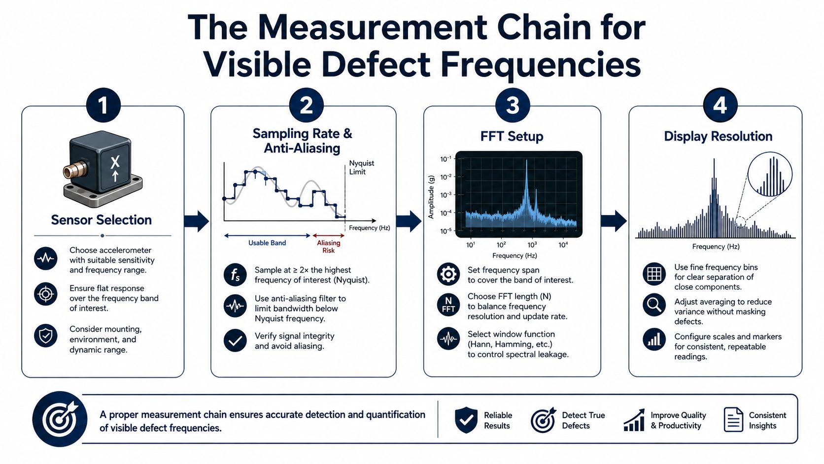
Settings that influence the result
- Windowing: Hanning works well for steady machinery. Uniform windowing can preserve transient amplitude when impacts are the target.
- Averaging: Linear averaging stabilizes periodic signals. Peak-hold preserves a transient peak that averaging could hide during a speed ramp.
- Mounting: A rigid, repeatable mount transmits high-frequency impact energy more consistently than loose contact or changing hand-held positions.
- Triggering and routing: Trigger timing and cable routing can reduce repeatability near variable-speed drives and strong electrical noise.
A route technician measuring a motor-driven pump should record speed, load, and operating condition with every spectrum. A reading taken at another speed or load is not a clean baseline, and fixed-hertz comparisons can mislead on variable-speed equipment. Use order-based comparisons where appropriate, then inspect harmonics and sidebands rather than accepting one cursor match. Reliable collection starts with practical vibration measurement guidance, while teams investigating pump equipment can also review how to detect pump faults with vibration analysis.
Using Envelope Analysis to Surface Hidden Bearing Impacts
A pump can show rising high-frequency vibration while its raw acceleration spectrum still lacks a clean BPFO or BPFI line. A developing spall produces brief impacts, and each impact excites a structural resonance in the bearing housing, casing, or sensor path. The FFT may therefore show a broad resonance band while the lower impact repetition rate stays difficult to identify.
Envelope analysis, also called demodulation, separates the resonance from the impact pattern. The analyst band-pass filters acceleration around a suitable structural resonance, rectifies the filtered waveform, then applies a low-pass filter. The resulting envelope tracks impact amplitude over time. Its spectrum can expose BPFO, BPFI, BSF, or FTF, along with harmonics and sidebands.
Selecting the demodulation band
On many industrial assets, a useful structural resonance falls between 500 Hz and 8 kHz. That range is a starting point, not a fixed prescription. Select a band that captures repeated impact energy while rejecting gear mesh, electrical noise, flow excitation, and unrelated broadband activity.
Use this sequence:
- Capture an acceleration spectrum with enough high-frequency bandwidth.
- Locate a resonant band containing repeatable impact energy.
- Apply a band-pass filter around that resonance.
- Demodulate the filtered signal and inspect its envelope spectrum.
- Compare the result with calculated orders, harmonics, sidebands, time waveform, and operating history.
A narrow filter can miss impacts when resonance shifts with load, temperature, or mounting. A wide filter can admit noise and create a plausible pattern unrelated to the bearing. Test another reasonable band when the first envelope result disagrees with the waveform or machine condition. Repeated harmonic families strengthen the diagnosis, while an isolated cursor match deserves caution.
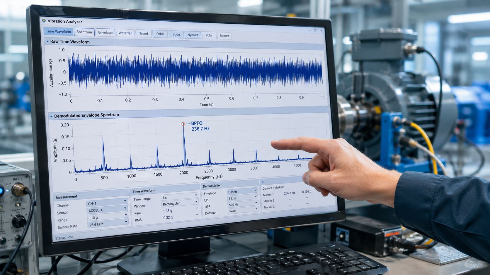
Envelope spectra can show sidebands spaced at shaft rate or cage frequency. That spacing helps separate a bearing impact train from random casing noise. An outer-race defect may remain subdued in the raw spectrum until direct tonal energy becomes severe, whereas demodulation can expose repeated impacts earlier. For broader time-series anomaly methods, see PlotStudio AI articles on anomaly detection. For the bearing-specific workflow, review vibration analysis for bearing fault detection.
Tracking Defect Frequencies Across Variable Speed Assets
A fixed FFT can mislead during a speed ramp. On a VFD-driven fan, compressor, or pump, the shaft accelerates while the analyzer collects the record. BPFO and BPFI move across frequency bins, and the impact train loses periodicity within the window. The result is often a smeared band rather than a clean defect line.
Order tracking keeps the measurement tied to shaft rotation. A tachometer or encoder supplies the speed reference, while synchronous resampling converts the time signal into the angle domain. BPFO, BPFI, BSF, and FTF can then appear as stable running-speed orders during acceleration or deceleration.
Choosing the right method
| Operating condition | Preferred method | Why it works |
|---|---|---|
| Stable speed | FFT with a fixed frequency target | The defect line remains in a consistent frequency location |
| Ramp with a usable tachometer | Order tracking and synchronous resampling | Impacts align by shaft position |
| Ramp without clean tachometer data | Waterfall or spectrogram | Frequency movement remains visible over time |
| Speed and load changing together | STFT or wavelet scalogram | Time-frequency methods show transient changes and evolving bands |
A waterfall plot shows a peak moving as speed changes. A spectrogram, commonly based on the Short-Time Fourier Transform, shows when energy appears and how its frequency shifts. These views display speed variation, but they do not correct it. With a reliable tachometer signal, order tracking usually gives the cleaner diagnostic result.
The measurement chain still sets the limit. Missing keyphasor pulses, low encoder resolution, or a poorly mounted tachometer can corrupt resampling. VFD switching noise may also require retaining a suitable high-frequency demodulation band before converting the signal to orders. Confirm that the tachometer pulse train is stable before trusting a precise order peak.
Decision rule: Use a fixed FFT at steady state within ±2% speed. Switch to order tracking during ramps. Use STFT or wavelet scalograms when both speed and load vary.
Speed should be treated as a live diagnostic input, not a fixed chart value. Work on bearing diagnosis under changing operating conditions emphasizes recalculating characteristic frequencies at each speed and estimating instantaneous defect frequency during fluctuation. The research on bearing diagnosis under variable conditions supports that approach.
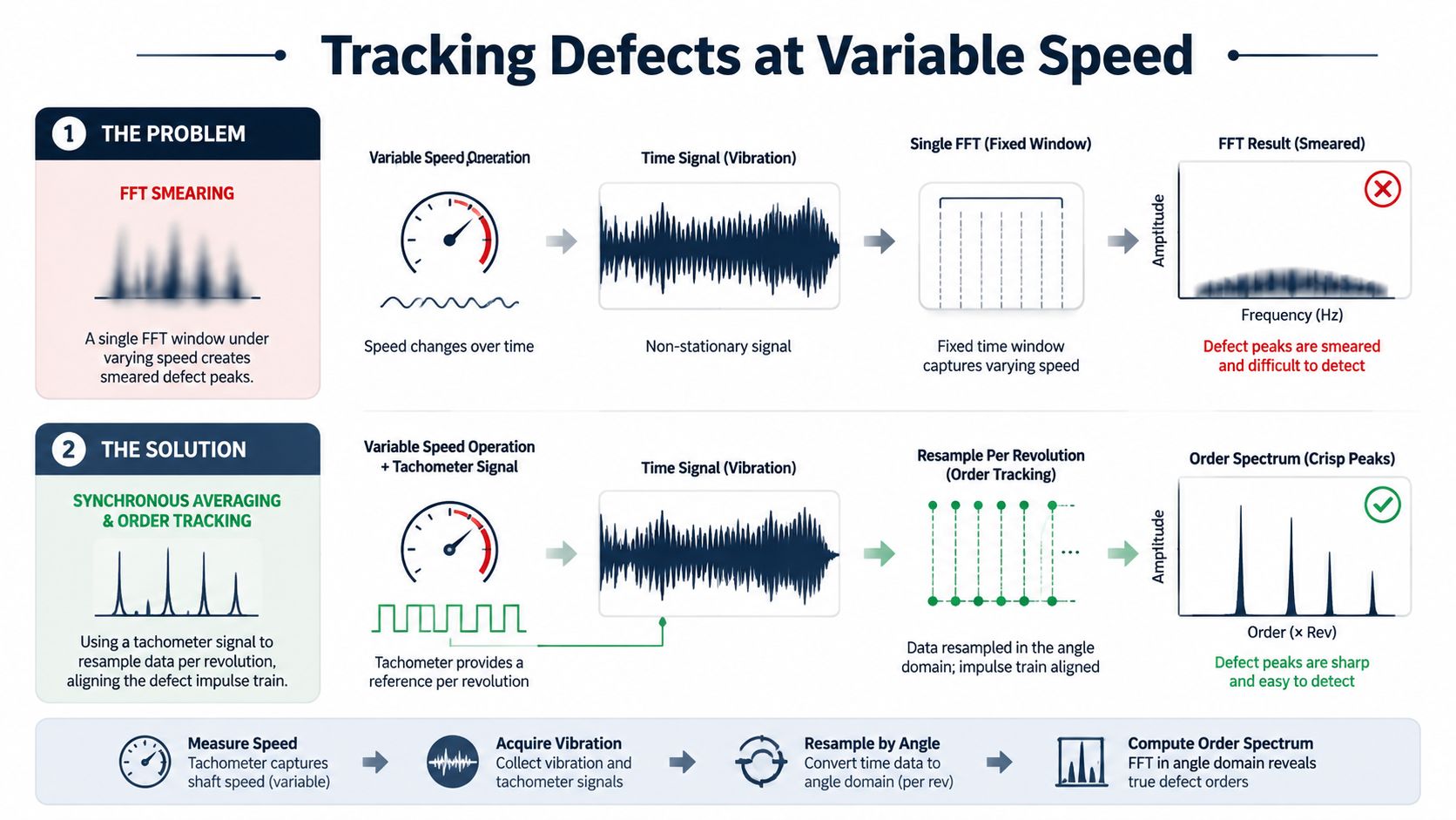
The practical check is agreement. A calculated order that remains aligned through the ramp, appears in the envelope result, and matches the time waveform deserves attention. A broad streak on a spectrogram or a single line from an unreliable speed reference does not establish a bearing fault. Recheck the tachometer, operating range, and resampling settings before making a maintenance decision.
Common Diagnostic Pitfalls When Reading Bearing Spectra
On a recent fan inspection, a BPFO-like peak proved to be a structural mode excited by motor electrical forces. The line matched the calculated frequency, but it did not behave like a bearing fault across operating conditions. That distinction prevents a frequency match from becoming an unnecessary work order.
Four traps recur on plant equipment:
- VFD switching artifacts: Electrical components can resemble bearing harmonics. If conditions permit, compare spectra with the drive in a different state. Then check whether the suspected family follows shaft speed or switching behavior.
- Structural resonance: Broadband impact energy can excite a casing mode that resembles a bearing tone. Compare the line with modal information, measurement position, and equivalent machines before assigning it to BPFO or BPFI.
- Ball slip: Slip shifts the actual defect rate away from the ideal calculation. Review bearing geometry, load, lubrication, and speed before rejecting a displaced line or forcing it to fit the formula.
- Single-peak confirmation bias: One strong line is weak evidence when it lacks harmonics, sidebands, trend growth, temperature change, acoustic evidence, or time-waveform support.
Envelope results deserve the same scrutiny. A true localized defect often produces a family of harmonics, while load-zone changes, impact transmission, and resonance can alter which harmonics dominate. Sidebands may support a bearing interpretation, but they can also reflect modulation from adjacent components or machine forces. Check the time waveform and measurement location rather than reading the spectrum in isolation.
Require at least two corroborating indicators before recommending replacement. A rising envelope trend combined with a matching harmonic family is stronger than either result alone. A physical listening check, temperature observation, lubricant review, and teardown evidence help separate a bearing fault from a transfer-path problem.
Severity also needs a consistent framework. The alert depends on asset criticality, baseline behavior, measurement method, and plant risk, not a universal amplitude copied from another machine. For vibration severity context and measurement discipline, teams can consult ISO vibration standards guidance.
A second look costs less than an unnecessary outage. It also reduces the chance of dismissing a genuine defect because the first spectrum was interpreted too narrowly.
Pump Bearing Case Study From First Alert to Replacement
The centrifugal pump entered alarm on a 2 g overall velocity alarm. Its envelope spectrum then developed activity near BPFI harmonics at multiples of 142 Hz, while BPFO sidebands spaced at shaft speed pointed to modulation linked to the race geometry. That combination set the diagnostic path, but the team still needed to establish whether the pattern was progressing.
Over the next six weeks, overall vibration doubled, and demodulated RMS rose steadily. Bearing-housing temperature also increased slightly, providing a physical indication that the condition was changing. The trend gave the reliability team a basis for planning work instead of reacting to one measurement.
Verification before the work order
The team examined the likely failure mechanisms and checked whether the spectrum matched the machine's physical condition:
- Oil analysis showed normal wear-particle counts, reducing the likelihood that abnormal lubrication debris was driving the signal.
- A manual listening check found irregular roughness at the bearing housing.
- The envelope pattern continued to show a raceway-related family of harmonics and sidebands as the pump condition worsened.
- The maintenance decision followed the plant's 8 g alert threshold for envelope amplitude.
The bearing was replaced after envelope amplitude exceeded that threshold. Teardown found an outer-race spall. The spectrum had contained BPFI harmonics and BPFO sidebands, so forcing the result into one isolated frequency would have obscured the actual defect pattern.
The post-replacement review focused on recurrence controls: fit, alignment, loading, lubrication, installation practice, and contamination exposure. Correct bearing geometry and installation matter as much as the diagnostic call. Teams can use this bearing selection and installation for maximum life reference to connect the finding with those controls before the pump returns to service.
Field Diagnostic Checklist for Reliability Teams
A reliable checklist turns a promising spectrum into a defensible maintenance decision. Start with the bearing identity, then verify the measurement and operating conditions. Formula accuracy matters, but it cannot correct the wrong bearing geometry or a reading taken during an unrepresentative load or speed.
Before collecting data
- Confirm the bearing: Record the complete part number, rolling-element count, contact angle, and pitch diameter. Calculate BPFO, BPFI, BSF, and FTF before visiting the asset, and note that these values are estimates when speed or geometry is uncertain.
- Set the acquisition chain: Set Fmax at least 10× the expected defect frequency and sample above 2.56× Fmax. Use Hanning windowing and collect three to five averages when a stable spectrum is needed. On variable-speed equipment, record running speed with each measurement.
- Demodulate the impacts: Choose a band-pass region around the structural resonance that carries bearing impacts. Inspect the envelope spectrum for the predicted frequency family, harmonics, and shaft-synchronous sidebands. A clean line in the raw spectrum is not required for a useful demodulated result.
- Trend the evidence: Track BPFO, BPFI, BSF, and FTF amplitudes with overall vibration, temperature, speed, and load. Look for a consistent change across readings rather than treating one peak as a replacement decision.
- Verify the operating story: Check lubrication, contamination, alignment, load zone, speed changes, and recent process modifications. Confirm that the sensor location and mounting method have stayed consistent.
If exact geometry is unavailable, document the assumptions and the speed used for each calculation. A practical bearing-failure workflow can trend narrow bands around BPFO, BPFI, and BSF at 1×, 2×, and 3× the fault frequency with a ±5% window. This approach follows predicted frequency regions instead of depending on one FFT bin. The bearing-failure study describing these frequency-domain features describes this measurement approach.
Forge Reliability provides vibration analysis, condition monitoring, and reliability consulting for industrial assets, including route-based and continuous monitoring programs. An outside review can help determine whether bearing diagnostics account for geometry, speed variation, envelope settings, and root-cause controls.
Forge Reliability can assess critical bearing assets and review BPFO, BPFI, BSF, and FTF practices. Visit Forge Reliability to request a free reliability assessment.