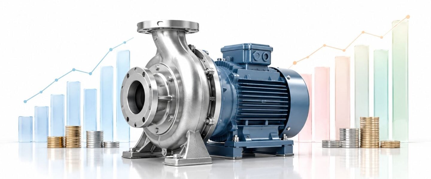
A maintenance manager approves a low-bid centrifugal pump because the price looks right and the spec sheet checks the boxes. Fourteen months later, the seal starts leaking, vibration climbs, the inboard bearing runs hot, and the night shift calls in overtime to swap parts and get production back. The purchase price was cheap. The asset wasn't.
That pattern shows up in plants with packed criticality lists. One pump doesn't fail alone. It drags maintenance labor, spare parts, production scheduling, and operator confidence with it. In a facility with more than twenty critical assets, repeated failures on even one machine can distort the maintenance budget and force capital decisions under pressure instead of by plan.
That's where life cycle cost analysis stops being a finance exercise and starts becoming a reliability tool. The useful question isn't “What does this pump cost to buy?” It's “What will this pump cost to own, maintain, and recover from when it fails in this duty?”
A reliability team already has most of the raw material needed to answer that. CMMS work orders show repeat failure modes. Vibration routes show bearing condition trends. Oil analysis flags contamination and wear. Thermography catches thermal imbalance. Ultrasound helps confirm lubrication and air leak issues. When those condition inputs are tied to cost and timing, the repair-versus-replace decision gets much sharper.
A strong foundation for recurring pump problems is disciplined failure elimination, and a practical reference on that topic is centrifugal pump reliability and failure prevention.
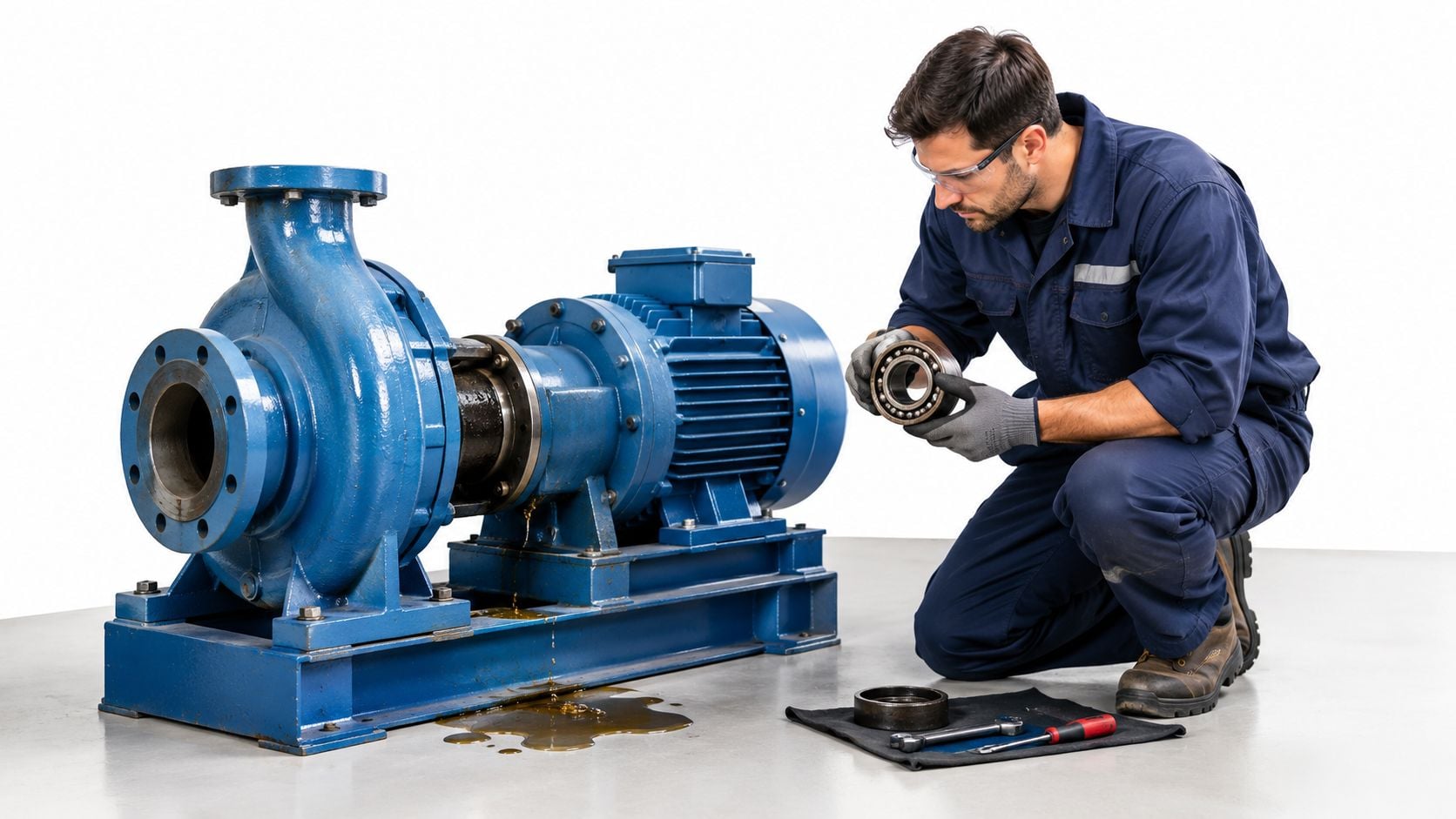
Table of Contents
- Introduction When the Cheapest Pump Becomes the Most Expensive
- What Life Cycle Cost Analysis Really Means for Industrial Assets
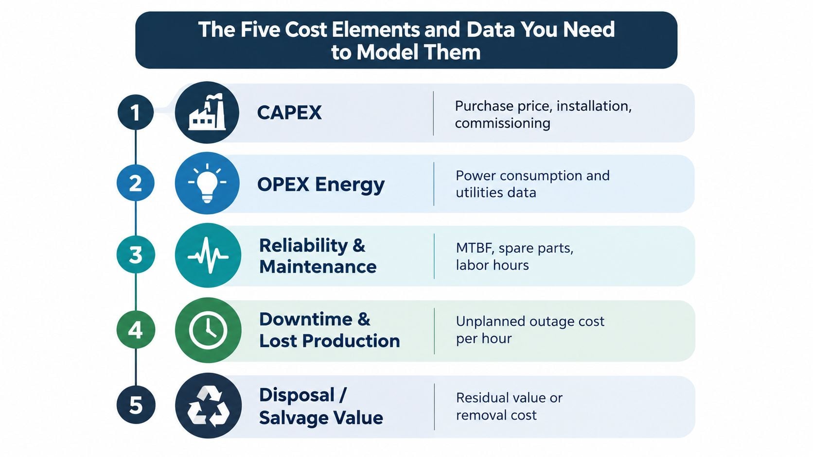
- The Five Cost Elements and Data You Need to Model Them
- How to Build a Life Cycle Cost Model Step by Step
- Modeling Approaches Sensitivity Analysis and Uncertainty
- Example Calculations for Pumps and Motors and Repair vs Replace Decisions
- Common Pitfalls and How LCCA Improves Capital Planning
Introduction When the Cheapest Pump Becomes the Most Expensive
A leaking seal rarely stays a seal problem. On a process pump, leakage often comes with shaft movement, bearing distress, coupling misalignment, pipe strain, or poor lubrication practice. If the plant keeps treating each event as an isolated repair, the accounting system spreads the pain across labor, stores, and lost throughput, and ownership cost stays hidden.
That's why plant leaders often get confused by “cheap” equipment. The invoice is visible on day one. The reliability penalty arrives in fragments over the next several shutdowns.
What usually gets missed
Most plants already count parts and labor. Fewer plants assign the full operational consequence of failure to the asset decision. A recurring seal failure can trigger:
- Overtime labor: Emergency callouts, rushed alignment, and extra supervision.
- Spare parts churn: Mechanical seals, bearings, sleeves, gaskets, and coupling elements leave the storeroom faster than planned.
- Production instability: Operators throttle around weak equipment, process conditions drift, and upstream or downstream assets absorb the upset.
- Planning disruption: The weekly schedule turns reactive because one bad actor keeps taking priority.
The cheapest machine on the bid tab often becomes the most expensive machine on the route.
What a plant leader needs from the analysis
A useful life cycle cost analysis should help answer practical questions:
- Should the plant repair the existing asset again, replace it, or change the design?
- Which failure costs belong in the model, and which ones are just noise?
- How should failure timing from Weibull analysis change the expected cost curve?
- When does predictive maintenance create a measurable financial difference in the model?
Those questions lead straight into the definition of the method.
What Life Cycle Cost Analysis Really Means for Industrial Assets
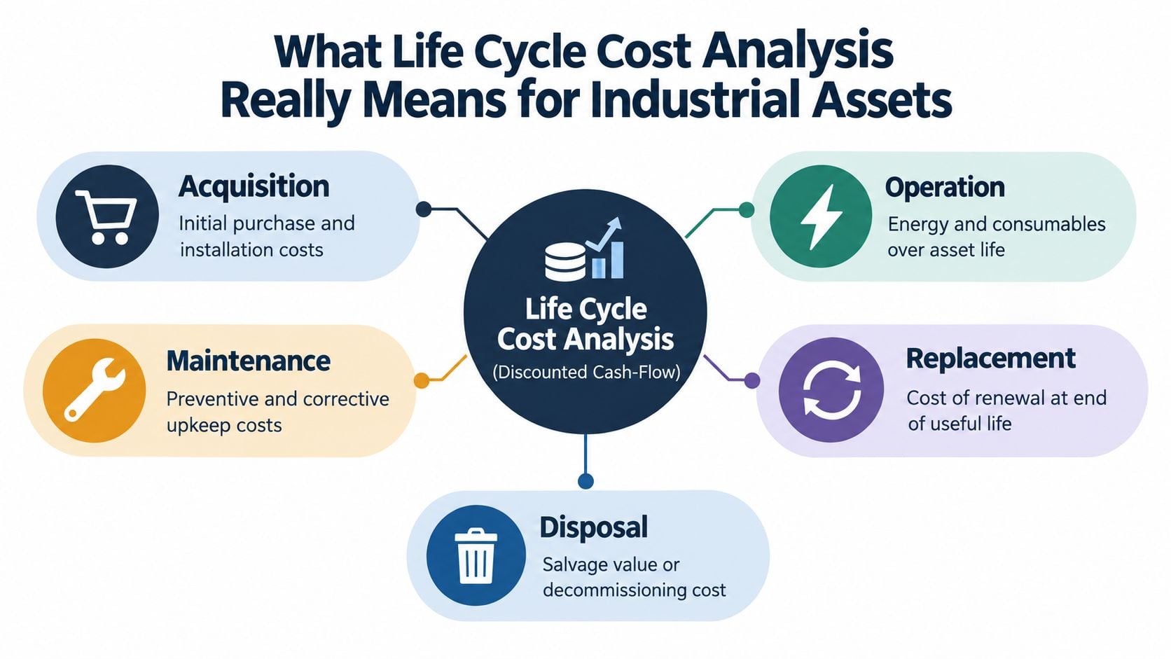
For industrial assets, life cycle cost analysis means comparing options over the full working life of the equipment, not just at the time of purchase. NIST defines life-cycle cost as a discounted cash flow method that totals acquisition, operation, maintenance and repair, replacement, and disposal costs over a defined study period in NIST Handbook 135. On the plant floor, that matters because the largest difference between two pumps or motors often shows up years after startup, inside failure, downtime, and maintenance spending.
A pump purchase works like buying a truck for a delivery fleet. The sticker price matters, but fuel burn, tire wear, breakdown frequency, and time out of service often decide whether that truck was the low-cost choice. Industrial assets follow the same pattern. The invoice is only the entry point.
The terms that matter on the plant floor
Three terms create most of the confusion, and each one has a practical meaning.
- Study period: The time window used to compare alternatives. It must be long enough to capture the failure behavior that separates one option from another. For a motor, that may mean several repair cycles. For a pump in abrasive or cavitating service, it may need to include major overhaul or replacement timing.
- Discount rate: The rate used to convert future cash flows into today's dollars. In plain terms, a dollar spent six years from now does not weigh the same as a dollar spent during this shutdown.
- Net present value or NPV: The present value of all relevant cash flows added into one number for each option, so repair, replace, or redesign choices can be compared on the same basis.
Plant leaders do not need to become finance specialists to use LCCA well. They need one discipline. Put every meaningful cost on the same time basis, then compare alternatives without mixing year-one dollars with year-seven dollars.
Why reliability belongs inside the cost model
This is the point many spreadsheet-only analyses miss. In an industrial plant, cost does not arrive as a smooth annual average. It arrives as failure events. A seal leak, bearing failure, rotor rub, or winding fault creates a burst of labor, parts, lost production, contractor time, and schedule disruption. If those events are frequent, early, or both, the NPV changes fast.
That is why LCCA becomes far more useful when it is built from reliability evidence rather than accounting categories alone.
A reliability-driven model asks four practical questions:
- How often is the asset likely to fail?
- What does each failure event cost to repair and recover from?
- When in the asset life do those failures tend to occur?
- Can predictive or condition-based work prevent part of that cost?
Where Weibull, CMMS history, and predictive maintenance fit
Weibull analysis estimates how failure probability changes with age or operating time. CMMS history gives the raw field record, work orders, parts usage, labor hours, and repeat failure patterns needed to estimate real repair cost and event frequency. Predictive maintenance savings enter the model as avoided failures, reduced outage duration, or shifted intervention timing.
Put those three together and LCCA stops being a finance exercise that happens after the technical decision. It becomes the technical decision, translated into money.
For example, if CMMS records show a pump family repeatedly loses seals between planned outages, Weibull analysis can help estimate when the next failures are likely to cluster. Those expected events can then be placed into an NPV model for two choices: keep repairing the current design or replace it with a design that costs more up front but fails less often. If vibration monitoring or oil analysis can catch deterioration early enough to avoid emergency work, the savings belong in the model too, because they change both failure timing and failure consequence.
Practical rule: The option with the lowest purchase price rarely stays cheapest if it produces more failure events, earlier failure events, or longer outages.
A useful introductory life cycle cost analysis example can help frame the basic logic. In asset-intensive plants, the analysis gets stronger when it is tied to failure distributions, cleaned CMMS records, and a formal asset lifecycle management framework that connects maintenance strategy, replacement timing, and risk.
The Five Cost Elements and Data You Need to Model Them
Most weak models don't fail because the math is difficult. They fail because the inputs are incomplete, inconsistent, or detached from failure behavior. A plant can build a polished spreadsheet and still make a bad replacement decision if the downtime cost is omitted or the CMMS history isn't cleaned up.
The five cost elements below are the core structure for industrial assets.
Cost element one through three
Acquisition cost includes purchase, installation, baseplate work, alignment, commissioning, piping modifications, electrical changes, and startup support. For a replacement pump, this also includes the cost of planned outage work needed to install it correctly.
Operating cost covers the energy and consumables required to run the asset. On a pump, that may include power draw, seal flush consumption, and utility support tied to the operating profile. On a motor, energy losses tied to degraded condition or loading profile can matter over the study period.
Reliability and maintenance cost is where most plant decisions become technical. This bucket includes preventive tasks, corrective repairs, labor hours, spare parts, contractor support, inspections, and repeat interventions linked to known failure modes.
Cost element four and five
Downtime and lost production cost should reflect the operational consequence of failure, not just the maintenance craft time. A failed feed pump can starve an entire line. A motor failure on a redundant auxiliary may have much lower consequence. Same repair labor. Very different business impact.
Disposal or salvage value often gets skipped because it sits late in the timeline. It still belongs in the model. Removal cost, scrap handling, environmental disposal, or residual value should be included if they differ meaningfully between options.
Hidden costs usually enter through the back door. They show up as expediting, temporary workarounds, rushed rentals, and repeated troubleshooting time that never gets coded cleanly.
Where the data should come from
A plant already has more data than it thinks. The challenge is connecting it.
- CMMS history: Work orders, failure codes, labor hours, parts usage, repeat defect patterns, and backlog notes.
- Vibration analysis: Bearing defect trends, imbalance, misalignment, looseness, hydraulic instability signatures, and resonance clues.
- Oil analysis: Viscosity change, contamination, wear debris, and lubricant condition that affect failure progression.
- Thermography: Thermal imbalance, overloaded connections, cooling restrictions, and friction heating.
- Ultrasound: Lubrication quality, friction onset, steam trap behavior, compressed air leakage, and some bearing distress indicators.
- Weibull analysis inputs: Time-to-failure data grouped by consistent failure mode and operating context.
- Criticality ranking: Consequence of loss, detectability, redundancy, and process exposure.
A practical readiness check
Before building the model, the team should verify:
- Failure modes are separated. Seal failures, bearing failures, and cavitation damage shouldn't be blended into one generic “pump failure” bucket.
- Work order closeout quality is usable. Free-text chaos weakens every cost estimate.
- Operating context is known. Duty cycle, process fluid, starts and stops, and standby versus continuous service all affect interpretation.
- Condition data is time-aligned. Diagnostic findings should connect to the period before failure or intervention.
- Production consequence is agreed with operations. Maintenance alone can't set this assumption.
Plants trying to connect maintenance cost to reliability planning often formalize this work through reliability-focused maintenance budgeting, because budget discipline improves when failure cost is tied to asset behavior instead of to last year's spending.
How to Build a Life Cycle Cost Model Step by Step
A good model compares alternatives, not isolated facts. In oil, gas, and pipeline applications, ISO 15663 frames life cycle costing as a way to compare competing options across project phases rather than to estimate the standalone cost of one piece of equipment in ISO 15663 guidance. That framing translates well to manufacturing and process plants because the actual decision is usually between options such as repair, replace, redesign, or operate-to-failure with contingency.
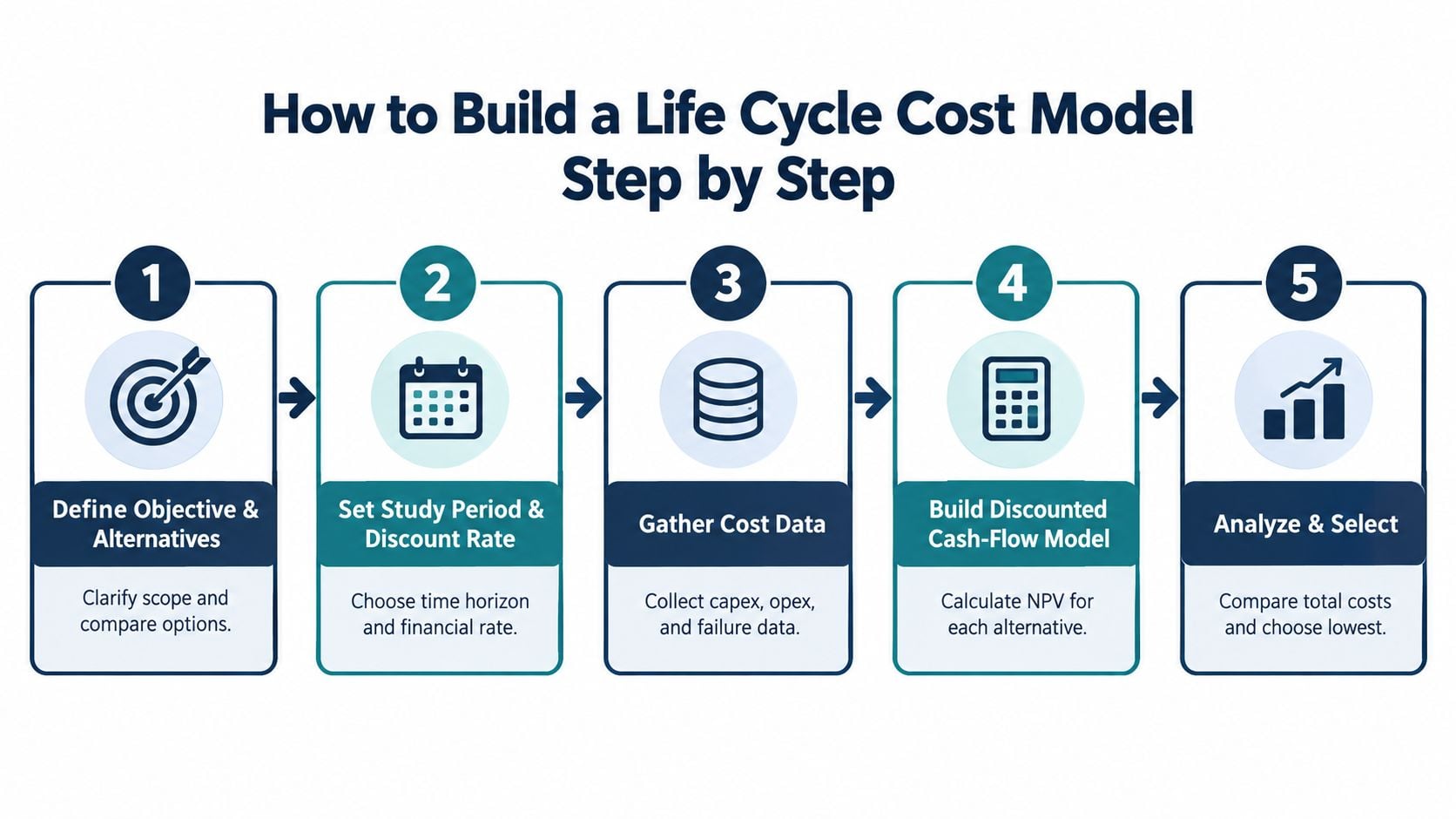
Step one and two
Define the decision objective. For a recurring pump problem, the alternatives might be: continue current repair practice, upgrade seal system and bearing housing, replace with a heavier-duty pump, or modify the process duty so the machine operates closer to best efficiency.
Set the scope and study period. A single-asset scope works when the failure consequence is local and the equipment operates largely independently. A whole-system scope works better when one machine drives line throughput, utility balance, or product quality.
ISO 15663-1 describes the method as the systematic and iterative consideration of differences between costs and revenues for alternative asset options, including estimating, planning, monitoring, and discounting cash flows to a base period in ISO 15663-1. The words systematic and iterative matter. The model should be revised as field data improves.
Step three and four
Lay out cash flows by year. Capital work usually lands early. Energy, routine maintenance, and expected corrective events spread across the study period. Major replacement or overhaul goes into the year it's expected to occur.
Choose the comparison method. Most plant teams use NPV because it keeps the alternatives comparable in present-value terms. Some also annualize the result to support budget planning, but the decision logic still starts with discounted cash flow.
Step five
Integrate failure behavior, not just average cost. The reliability function enters. Weibull analysis helps estimate how failure likelihood changes with time. A wear-out pattern doesn't behave like random infant mortality or sporadic process abuse. The expected corrective maintenance cost should reflect that shape.
For example, if a motor bearing population shows age-related wear-out, the model can place higher expected repair exposure later in the study period instead of spreading it evenly. If a pump seal failure is driven by frequent starts and dry-run events, operations may need to validate whether those starts will continue before the model locks in assumptions.
A life cycle cost model is only as credible as the operating assumptions signed off by production, maintenance, and engineering together.
When to use system scope instead of machine scope
Use a broader frame when the asset is tightly coupled to the process:
- Pumps: Shared suction conditions, process hydraulics, and standby logic can change the economics.
- Compressors: Throughput, energy, and process constraints often dominate the decision.
- Motors and gearboxes: If they drive bottleneck equipment, local repair cost is often less important than production consequence.
ISO 15663-2 notes that the methodology is intended for facilities in drilling, production, and pipeline transportation, and also notes that it isn't about calculating the life-cycle cost of individual items of equipment in ISO 15663-2. In plant practice, that's a useful reminder not to over-isolate a machine whose true cost sits in the system around it.
Clean year-by-year cost data often starts with disciplined work order and asset hierarchy structure in the CMMS and asset management process.
Modeling Approaches Sensitivity Analysis and Uncertainty
A deterministic model uses one assumed value for each input. One failure interval. One discount rate. One maintenance cost. One energy price. That's simple, and it's often the right starting point. It's also where many teams become overconfident.
A methodological review highlighted hidden costs, uncertainty of future costs, and discounting as unresolved issues, and more recent guidance has pushed sensitivity, risk, and uncertainty analysis into standard practice in this life cycle costing review. For industrial assets, that's not academic. Failure timing, labor variability, inflation, and downtime consequence rarely hold still.
Deterministic versus probabilistic thinking
A deterministic spreadsheet is useful when the failure mechanism is stable and the consequence range is narrow. A non-critical utility pump with consistent maintenance history may fit that pattern.
A probabilistic approach is stronger when the plant is dealing with uncertain failure timing, changing duty cycle, or hidden costs such as obsolete spares and variable outage duration. In that case, the team models a range of outcomes instead of one single line of certainty.
What to test first
Sensitivity analysis should target the variables most likely to move the decision:
- Failure timing: Often estimated from Weibull analysis or grouped history.
- Downtime consequence: Especially where process interruption ripples into multiple units.
- Energy cost exposure: More relevant for continuously loaded motors, fans, and pumps.
- Corrective repair scope: Parts-only assumptions often understate total event cost.
- Condition-based maintenance savings: If predictive tasks catch defects earlier, the event cost and timing can both change.
A practical guide on sensitivity versus scenario testing that helps teams avoid costly modeling mistakes can be useful when choosing whether to vary one input at a time or test bundled operating scenarios.
The gap in current practice
An integrative review argues that life cycle cost analysis still lacks a mature, integrated decision-support framework that combines use profile, energy-efficiency retrofits, and optimized maintenance and resource management in the 2025 review on LCCA methodology. That gap matters in plants because machines rarely live in static conditions. Throughput changes, product mix changes, and maintenance strategy changes all shift the cost picture.
One practical response is scenario testing. Build one case for current operation, one for increased duty, one for maintenance improvement, and one for deferred capital replacement. Then compare which assumptions swing the answer. A team that needs structured Weibull inputs for that work may use Weibull analysis software or an equivalent internal method to make the failure timing assumptions explicit.
Example Calculations for Pumps and Motors and Repair vs Replace Decisions
The model becomes useful when it changes a real decision. Consider two common plant problems: a centrifugal pump with recurring mechanical seal failures and a motor showing insulation deterioration through testing and operating history. The point isn't to produce a universal answer. The point is to show how year-by-year expected costs can be compared in one framework.
Pump example with recurring seal and bearing work
A process pump keeps failing through the same chain. Seal leakage starts first. Bearing temperature rises later. Vibration confirms developing bearing distress, and teardown repeatedly finds shaft movement and wear tied to alignment and hydraulic instability.
The team compares three options over a ten-year study period:
| Option | Capex | 10-Year NPV of O&M and Downtime | Total LCC |
|---|---|---|---|
| Repair existing pump as failures occur | Higher recurring corrective exposure | Highest expected value because failures continue | Highest |
| Replace with upgraded pump package | Higher initial outlay | Lower expected corrective and downtime exposure | Lower than reactive repair if failure pattern is persistent |
| Retrofit support systems and improve alignment, sealing, and operating practice | Moderate initial outlay | Middle range, depends on whether root causes are fully removed | Can be lowest if failure mode is truly design- or practice-driven |
No invented plant numbers are needed to see the logic. If the expected failure cost remains high and the outage consequence is severe, the “cheap” repair path often carries the highest total life cycle cost.
Motor example with insulation degradation
A large motor may not fail the way a pump does. The warning signs are different. Insulation resistance trends, thermal behavior, unbalance, current signature, contamination, and cooling effectiveness all matter. The question is often whether to rewind, replace, derate, or hold a strategic spare while condition monitoring continues.
A published ASME gas turbine study shows the basic logic clearly. Lifecycle cost analysis combines initial equipment cost with fuel, labor, and parts, and another gas turbine study calculates each cost as net present value before summing them into a lifetime NPV in the ASME lifecycle cost paper. The same structure translates to motors. Replace “fuel” with energy and production consequence, and the framework still works.
Where Weibull changes the decision
If the pump's failure data shows a wear-out pattern, expected corrective cost should rise as the machine ages unless design changes break the pattern. If the motor's condition data suggests increasing likelihood of winding failure under continued duty, the cost of deferral should be weighted more heavily in later years.
That changes repair-versus-replace logic in practical ways:
- Choose repair when the failure mode is isolated, consequence is manageable, and corrective cost doesn't trend upward sharply.
- Choose retrofit when diagnostics point to removable causes such as misalignment, lubrication problems, pipe strain, contamination, or control issues.
- Choose replacement when repeated failures reflect fundamental design mismatch, obsolete supportability, or rising downtime exposure that maintenance can't reasonably control.
A plant may also use the same model for spares strategy. If a critical spare shortens outage duration enough to materially reduce expected consequence, stocking it may carry lower total cost than repeated exposure to long lead-time recovery.
Common Pitfalls and How LCCA Improves Capital Planning
The most common mistake is treating life cycle cost analysis as a one-time spreadsheet built for budget season. Asset behavior changes. Duty changes. Failure coding improves. A model that never gets updated turns into a false sense of rigor.
Another error is excluding downtime because it's “hard to estimate.” In many plants, that's the very term that separates a sensible repair decision from a damaging one. If the team ignores process consequence, the model can recommend the lowest invoice path while production keeps absorbing the penalty.
Four errors that quietly break the model
- Using cost averages without failure mode separation: Seal failures, bearing failures, and electrical failures shouldn't be pooled.
- Applying one fixed financial assumption with no challenge: If discount rate, repair scope, and outage duration never get stress-tested, the model may look precise while being fragile.
- Skipping end-of-life treatment: Removal, salvage, decommissioning, and residual value still affect the comparison.
- Ignoring data governance: CMMS coding discipline, asset hierarchy quality, and closeout consistency determine whether next year's model improves or degrades.
How the method strengthens capital planning
When maintained properly, life cycle cost analysis improves more than a single replacement decision. It helps plants:
- Prioritize capital by asset consequence and repeat failure economics
- Support spare parts optimization with consequence-based logic
- Link predictive maintenance findings to budget timing
- Improve OEE planning by reducing recurring reactive interruptions
One practical option for plants building this capability is to involve a specialist such as Forge Reliability for condition monitoring, Weibull analysis, and asset management support where internal data quality or reliability resources are still developing.
Capital planning gets better when engineering stops arguing from purchase price and starts arguing from expected failure cost.
The strongest programs treat LCCA as part of the asset management workflow. Reliability engineering supplies the failure behavior. Maintenance supplies work history and repair content. Operations supplies consequence and duty profile. Finance supplies the discounting discipline. When those pieces stay connected, repair-versus-replace decisions become easier to defend.
Forge Reliability helps industrial teams connect CMMS history, predictive maintenance findings, and failure analysis to practical asset decisions such as repair, replacement timing, and spare strategy. For plants that want a cleaner view of recurring failure cost and a stronger basis for capital planning, a free reliability assessment is a practical next step through Forge Reliability.