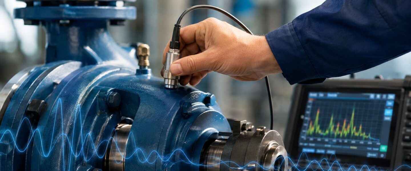
A centrifugal pump can pass every weekly route and still be moving toward failure. The usual problem isn't a lack of data. It's that the route captures one overall number, at one location, under one operating condition, while the actual fault is hydraulic, structural, directional, or hidden inside a bearing's high-frequency signal.
That distinction matters in cooling water, chemical processing, wastewater, oil and gas, and any plant where a pump trip interrupts production. Vibration analysis of pumps becomes useful when it connects a physical signal to a maintenance decision: continue operating, correct the process, inspect the machine, or schedule a repair.
Table of Contents
- The Pump That Looked Fine Until It Wasn't
- What Vibration Actually Tells You About a Pump
- Sensors, Mounting, Routes, and Sampling Done Right
- Reading the Spectrum Common Pump Fault Frequencies Explained
- Time Waveforms Enveloping and Broadband Energy
- Trending KPIs and Acceptance Criteria That Drive Action
- Two Pump Case Studies From the Plant Floor
- Turning Diagnostics Into Reliability Results
The Pump That Looked Fine Until It Wasn't
A 2,200 GPM centrifugal pump in cooling-water service had passed every weekly vibration route for nine months. Its velocity RMS remained comfortably inside ISO 10816-7 Zone B. The technician measured the motor, recorded an acceptable value, and moved to the next asset.
At 03:14 on a Sunday, the bearing housing tripped on high temperature. The coupling guard was cracked, and the pump was no longer available for service. The plant lost 38 hours of production, expedited a bearing exchange, and opened an incident report.
The failure didn't become inevitable at the moment of the trip. A radial load had been developing at the pump-end bearing for weeks, but the route measured in-plane velocity on the motor. A recirculation line two meters away masked the developing acoustic signal, and the handheld probe was repositioned slightly on each round. The data showed no impending failure because the measurement setup couldn't reliably observe it.
Practical rule: A pass or fail velocity value describes the measurement point and operating condition. It doesn't prove that every important pump failure mode is absent.
A useful diagnostic program would have compared the motor and pump bearing housings, captured radial and axial readings, recorded process state, and checked high-frequency energy. It would also have investigated whether vibration changed with flow, valve position, suction pressure, or recirculation.
That is the difference between collecting readings and diagnosing a machine. The first supports a route-compliance report. The second helps an engineer distinguish a defective bearing from a hydraulically unstable pump.
What Vibration Actually Tells You About a Pump
Every rotating pump produces a physical signal. The rotor, bearings, casing, coupling, foundation, and fluid interact, and that interaction creates movement that a sensor can measure. A useful analogy is speech: the machine is speaking, but each measurement method captures a different part of the message.
Three measurements, three diagnostic jobs
Displacement describes how far a shaft or casing moves, commonly in mils or micrometers. It's especially useful for slow-speed equipment, shaft-clearance questions, and evaluating movement at 1× running speed, where one cycle occurs per shaft revolution.
Velocity is measured in mm/s or in/s RMS. RMS means root mean square, a way of expressing the effective energy of an alternating vibration signal. Velocity is the common general-health metric for pump trains because it represents a broad portion of the frequency range where mechanical faults often appear.
Acceleration is measured in g RMS or g peak. It responds strongly to rapid impacts and high-frequency energy from rolling-element bearings, gear teeth, lubrication problems, and cavitation. Acceleration is also the usual input for envelope demodulation, a processing method that extracts repetitive impacts from a noisy vibration signal.
Sensor selection follows the suspected fault. A low-frequency shaft or structural problem needs a measurement setup with suitable low-frequency response. An early bearing defect needs enough high-frequency bandwidth and a mounting method that preserves the impact signal. Beginners often choose a sensor first and then ask what it can detect. The safer sequence is the reverse.
Why the same pump can show different answers
A motor-end reading may look normal while the pump-end bearing carries a growing hydraulic or mechanical load. An axial measurement may reveal coupling or thrust behavior that isn't visible in a horizontal radial reading. A casing measurement may show resonance or vane-pass excitation that doesn't resemble a bearing defect.
For teams building a bearing-focused route, a practical primer on pump bearing failure mechanisms helps connect the measured signal to the component at risk. The measurement only becomes valuable when the analyst can explain which force generated it and where that force travels through the machine.
Sensors, Mounting, Routes, and Sampling Done Right
Measurement quality starts before the analyzer records an FFT. An FFT, or Fast Fourier Transform, converts a time waveform into frequency components. If the sensor location changes, the mounting is inconsistent, or the sampling settings hide the suspected fault, a clean-looking spectrum can still be misleading.
Match the sensor to the fault
For pumps operating below 3,000 RPM, a 100 mV/g accelerometer provides useful low-frequency resolution when mechanical faults are suspected. For bearing or gear-mesh investigations above 5 kHz, a 500 mV/g or IEPE-style sensor with a flat response to 10 to 15 kHz is more suitable.
Mounting matters just as much. A stud-mounted accelerometer preserves the sensor's specified usable range. Epoxy or glued mounting reduces that range by roughly 30%, while a magnetic mount costs another 20% and should generally remain a route-measurement option. A handheld probe can work, but only when its repeatability has been verified and documented.
| Mount method | Usable range | Repeatability | Best use |
|---|---|---|---|
| Stud-mounted accelerometer | Closest to full sensor specification | Highest | Permanent monitoring and diagnostic captures |
| Epoxy or glued mount | Roughly 30% less than the stud-mounted range | Good when installed consistently | Semi-permanent points |
| Magnetic mount | Roughly 20% less than the epoxy-mounted range | Moderate | Route-based screening |
| Handheld probe | Depends heavily on contact technique | Acceptable only when verified | Quick route checks |
A team reviewing sensor types and application decisions can use this vibration analysis sensor reference when standardizing a route.
Build a route that can be repeated
For each bearing housing, capture two radial measurements and one axial measurement. Mark the orientation, use the same point every round, and log the sensor serial number and operator initials in the route file. On variable-speed pumps, allow the machine to pass through slow speeds before sampling so rotor float doesn't bias the reading.
Sampling must cover the highest frequency of interest. Set the sampling rate to at least 2.56 times that frequency. Choose an Fmax of 500, 1,000, 2,000, or 10,000 Hz, depending on the machine class and suspected fault. A Hanning window with 400 to 800 lines gives enough resolution to separate narrow peaks while retaining useful broadband information.
Process context belongs in the same record. Flow, suction pressure, discharge pressure, valve position, speed, and recirculation status can explain a vibration change that a spectrum alone can't. Teams designing that data workflow can also review this guide to IoT data analysis for broader principles around organizing sensor and process information.
Reading the Spectrum Common Pump Fault Frequencies Explained
A spectrum becomes easier to interpret when each peak is tied to a physical event. 1× running speed means one event per shaft revolution. 2× means two events per revolution. Vane-pass frequency comes from the impeller's interaction with the casing or diffuser, while bearing frequencies come from rolling geometry and shaft speed.
The working reference
| Fault Mode | Dominant Frequency | Typical Multiple | Key Clue |
|---|---|---|---|
| Unbalance | Running speed | 1× | Strong radial peak, often stable with speed |
| Misalignment or bent shaft | Running speed and harmonics | 2× is common | Axial vibration and phase relationship help separate causes |
| Electrical interaction | Line-frequency components | Multiples of line frequency | Peak changes with electrical condition or motor state |
| Hydraulic excitation | Vane-pass frequency | Number of impeller vanes × RPM | Changes with flow, valve position, or operating point |
| Mechanical looseness | Running speed harmonics | 1×, 2×, 3× and higher | Multiple harmonics, impacts, and unstable waveform |
| Rolling-element bearing defect | BPFO, BPFI, BSF, or FTF | Geometry-dependent | Repetitive impacts and envelope peaks |
| Cavitation | Broadband high-frequency energy | Often above 10× running speed | Hash-like spectrum, process dependence |
| Coupling wear | Running-speed harmonics and sidebands | Application-dependent | Directional or axial response, often with phase changes |
| Gear mesh | Gear-mesh frequency | Tooth count × shaft speed | Mesh harmonics and sidebands |
BPFO is the ball-pass frequency of the outer race. BPFI is the corresponding inner-race frequency. BSF refers to ball-spin frequency, and FTF is the fundamental train frequency associated with the cage. These frequencies don't equal a universal multiple because bearing geometry changes them.
For centrifugal pumps, cavitation often appears as broadband high-frequency energy above about 10× running speed, while a cited example places much of that energy in the 500 to 2,000 Hz band. Bearing defects instead produce characteristic frequency families tied to shaft speed. For a 1,800 RPM pump, example bearing bands can fall roughly between 80 and 150 Hz, depending on bearing geometry. These ranges are diagnostic clues, not automatic verdicts. This pump vibration frequency reference provides additional context for separating hydraulic and bearing signatures.
A 30-second FFT walkthrough
Consider a pump running at 1,800 RPM. Running speed is 30 Hz, so a dominant peak at 30 Hz points toward unbalance, shaft bow, or a force locked to rotation. A strong 60 Hz component, especially with axial response and phase changes across the coupling, raises misalignment or looseness concerns.
Suppose the impeller has six vanes. Vane-pass frequency would occur at 180 Hz. If that peak rises as flow moves away from the preferred operating point, hydraulic excitation becomes more credible than a new bearing defect. If the spectrum shows several harmonics of 30 Hz and an impact-rich time waveform, looseness deserves inspection.
A peak family around a bearing's calculated BPFO or BPFI, especially in an envelope spectrum, points toward a rolling-element defect. A broad rise across the high-frequency band without clean synchronous peaks points more toward cavitation, poor lubrication, or another impulsive process. The analyst should then compare the signal with pressure, flow, suction conditions, and operating point before issuing a work order.
Reliability teams applying standards to that interpretation can use this ISO vibration standards overview as a reference point, but standards don't replace machine-specific diagnosis.
Time Waveforms Enveloping and Broadband Energy
The FFT tells an analyst where energy sits in frequency. The time waveform shows how that energy arrives. That difference is essential when a pump has a quiet spectrum but a developing impact fault.
A clean sinusoidal waveform with gradually rising RMS often supports a progressive rotating force such as unbalance, or a developing wear process with a regular pattern. A clipped, distorted, or impact-heavy waveform raises concern about shaft rub, clearance impacts, mechanical looseness, or severe cavitation. The analyst should compare waveform shape at the motor, pump bearing housing, casing, and base rather than treating one point as representative of the entire train.
How envelope demodulation exposes hidden impacts
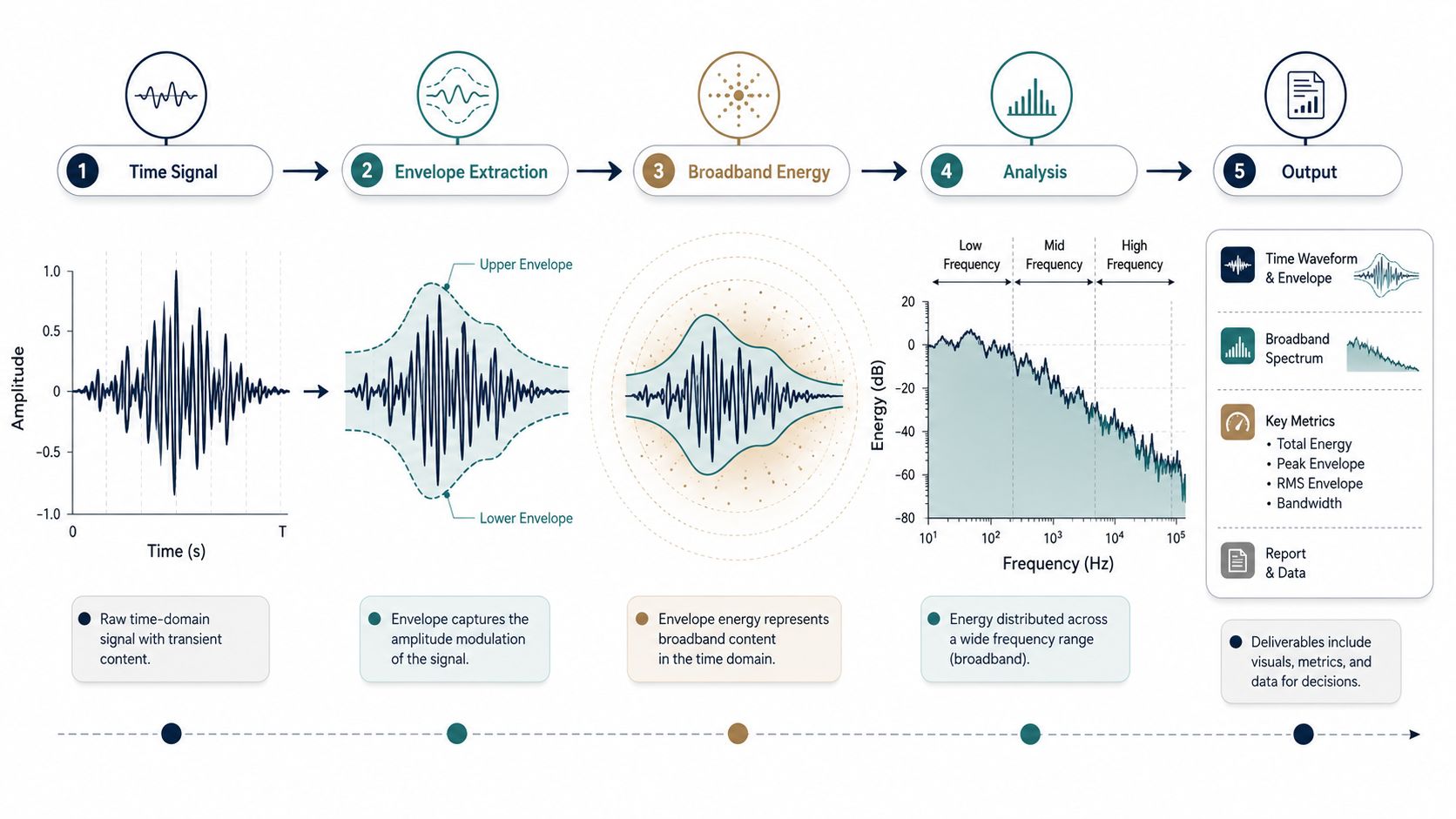
Early bearing defects can be buried beneath strong running-speed vibration. Envelope demodulation isolates them by applying a band-pass filter around a structural resonance, rectifying the filtered signal, and using a Hilbert transform to recover the repetition rate of the impacts. The resulting envelope spectrum can reveal BPFO or BPFI even when the ordinary velocity spectrum is dominated by 1× harmonics.
The method has trade-offs. A poorly selected filter band can suppress the fault or amplify unrelated noise. A magnetic mount can also weaken the high-frequency response, which is why diagnostic captures should use a consistent, rigid mounting method whenever practical. Teams selecting processing methods can consult this vibration analysis tools guide as part of a broader measurement standard.
Separate hydraulic noise from mechanical impacts
Cavitation often produces broadband energy and high-frequency kurtosis spikes. Kurtosis measures how strongly a signal is dominated by peaks compared with a more regular waveform. A high or rising value supports an impact-driven condition, but it doesn't identify cavitation by itself. Bearing defects, lubrication distress, rubs, and hydraulic instability can all create impulsive behavior.
The decision rule is simple: when the ordinary spectrum looks quiet, check the time-waveform crest factor, the envelope spectrum, and broadband energy. Then correlate the result with suction pressure, flow, valve position, and pump speed. A process-linked rise that disappears when the pump returns toward its intended operating point suggests hydraulic instability. A bearing-frequency family that persists across comparable operating states points more strongly toward mechanical damage.
Trending KPIs and Acceptance Criteria That Drive Action
A reliability program needs more than a severity chart. It needs KPIs that reveal both current condition and rate of change. The core set for pump trains includes overall velocity RMS, high-frequency band energy, gSE or envelope level, crest factor, kurtosis, and peak vibration at defined measurement points.
Use standards as boundaries, not diagnoses
ISO 10816-7:2009 formalized a dedicated vibration-evaluation framework for rotodynamic pumps in industrial applications with nominal power above 1 kW. It specifies measurements on non-rotating parts using RMS vibration velocity in mm/s and defines severity zones and limits for horizontal and vertical pumps. The framework was later extended through ISO 20816-5:2018 for hydraulic power generating and pump-storage plants, showing how pump assessment developed into a standards-based discipline over at least a 9-year period. The ISO 10816-7 standard reference is useful when a plant is defining measurement points and evaluation boundaries.
A widely used benchmark places newly commissioned motor-pump machinery at 1.4 mm/s RMS or less, unrestricted operation below 2.8 mm/s RMS, restricted operation from 2.8 to 4.5 mm/s RMS, and likely damage above 4.5 mm/s RMS. These values support decisions, but they don't tell the analyst whether a restricted reading comes from cavitation, misalignment, looseness, resonance, or bearing damage. This ISO vibration severity chart gives the cited benchmark.
For petroleum, petrochemical, and natural-gas service, API 610 sets a different acceptance framework. Within the preferred operating region, overall bearing-housing vibration is limited to 3.0 mm/s RMS for pumps running up to 3,600 r/min and absorbing up to 300 kW per stage. Discrete-frequency vibration is limited to 2.0 mm/s RMS, and shaft vibration is capped at 50 µm peak-to-peak for relevant configurations. The API 610 specification should govern contractual acceptance where it applies.
API 610 permits roughly a 30% increase in allowable vibration when operation remains within the allowable operating region but outside the preferred region. That allowance isn't permission to ignore a marginal operating point. It supports a controlled decision about whether to correct flow conditions, change the process, or schedule intervention. This API 610 vibration-limits discussion addresses that distinction.
Build an alert ladder
| Measurement | Standard | Acceptance Limit | Trigger Action |
|---|---|---|---|
| Overall bearing-housing velocity | ISO benchmark | Below 1.4 mm/s RMS for newly commissioned machinery | Establish baseline and verify route repeatability |
| Overall velocity | ISO benchmark | Below 2.8 mm/s RMS for unrestricted operation | Continue trending and investigate meaningful changes |
| Overall velocity | ISO benchmark | 2.8 to 4.5 mm/s RMS | Restrict operation as appropriate and plan corrective action |
| Overall velocity | ISO benchmark | Above 4.5 mm/s RMS | Remove from service as soon as possible when safe and practical |
| Bearing-housing velocity | API 610 | 3.0 mm/s RMS in the stated preferred-region application | Review acceptance, operating region, and mechanical condition |
| Discrete-frequency vibration | API 610 | 2.0 mm/s RMS | Identify the peak source before accepting the machine |
| Shaft vibration | API 610 | 50 µm peak-to-peak for relevant configurations | Escalate shaft and rotor evaluation |
The plant's own baseline should remain the first alarm reference. A practical ladder can use green for stable baseline behavior, yellow for a rise toward the ISO Zone B boundary or approximately 1.5 times baseline, and red for Zone C or D behavior or a rapid increase. The numeric trigger must be linked to a defined action, not merely displayed on a dashboard.
A rising envelope trend should prompt confirmation captures, operating-state checks, and, where justified, borescope inspection or a planned bearing review. Sustained broadband RMS should trigger a work-order review that includes suction conditions, recirculation, valve position, alignment, and structural checks. Maintenance leaders tracking these decisions can also use this reliability metrics guide to connect condition indicators with program performance.
Two Pump Case Studies From the Plant Floor
A chemical-plant centrifugal pump repeatedly appeared on the DCS trip log with cavitation alarms. Route spectra showed broadband energy between 200 and 800 Hz, but no dominant 1× or 2× peaks. Because the signal followed the hydraulic event rather than a rotating-frequency family, the team inspected the suction side instead of immediately replacing bearings. A partially blocked strainer was found, and the team verified the available NPSH margin after cleaning and restoring the suction path.
The maintenance decision was process correction, not a rotating-element overhaul. That distinction avoided using vibration as a catch-all diagnosis and directed the work toward the condition creating the instability.
A wastewater pump presented the opposite problem. Overall velocity remained inside ISO 10816-7 Zone B, yet a slow-developing outer-race defect was hidden beneath strong 1× harmonics. High-frequency envelope demodulation with a 1 kHz filter exposed BPFO impulses, allowing the team to schedule a bearing replacement rather than wait for an overall RMS alarm.
These cases show why a single KPI can't carry the entire program. Hydraulic instability often changes with flow, suction conditions, and control-valve position. A mechanical defect tends to maintain a component-related signature across comparable operating states, even when its contribution to overall velocity remains modest.
Turning Diagnostics Into Reliability Results
A spectrum has no reliability value until it creates a controlled action. Each confirmed fault should generate a work order, a root-cause review, a failure-mode update in the CMMS, and a revised preventive-maintenance task. If cavitation recurs, the failure record should preserve suction conditions and operating point, not just the phrase “high vibration.”
Maintenance leaders should escalate beyond in-house capability when the team faces repeated false positives, unfamiliar signatures, disputed post-overhaul baselines, or safety-critical equipment. Route consistency, analyst training, and independent review matter most when a pump's vibration is affected by both process behavior and mechanical condition.
A practical preventive-maintenance program also depends on clear technician tasks, documented inspection points, and actionable escalation rules. The WaterJobsIntel preventive maintenance guide offers useful context for structuring that work.
Forge Reliability provides vibration analysis and condition-monitoring programs for pumps, including route-based and continuous approaches, with diagnostic support for hydraulic and mechanical failure modes. A free reliability assessment can benchmark current routes, alarm zones, and corrective-action turnaround against ISO 10816-7 and applicable API 610 expectations.
Forge Reliability can review a plant's pump routes, sensor mounting, alarm strategy, and process-context data to separate hydraulic instability from true mechanical defects. Visit Forge Reliability to request a free reliability assessment and establish a defensible action plan before the next unplanned pump trip.