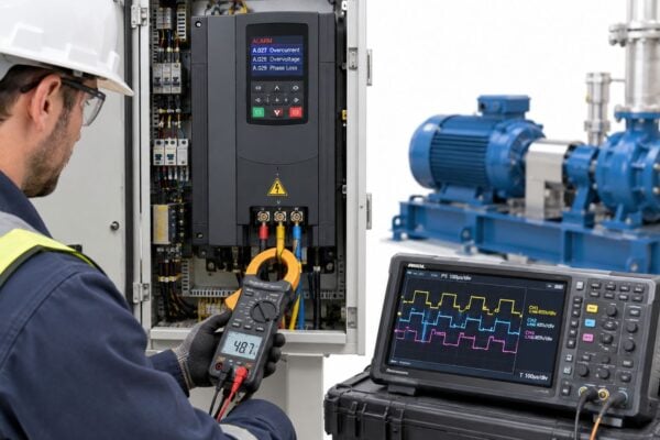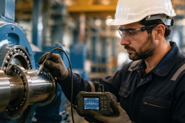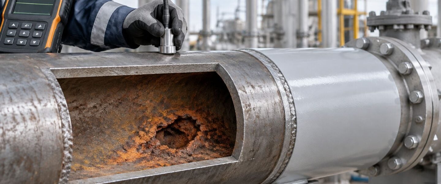
In 2025, internal corrosion accounted for 38% of all pipeline leaks and ruptures reported in Alberta, according to the Alberta Energy Regulator data. That share reframes corrosion in pipes as a detection problem, not only a materials problem. A line can retain acceptable average wall thickness and still contain one pit, groove, or concealed patch that reaches its limit first.
Reliable control therefore starts before the instrument purchase. Maintenance teams need to rank corrosion circuits, match the mechanism to the location, inspect where water and turbulence concentrate damage, and convert sparse readings into a defensible remaining-life decision.
Table of Contents
- Why Pipe Corrosion Costs More Than Its Rate Suggests
- Corrosion Mechanisms and the Failures They Cause
- What Drives Internal Corrosion in Process Piping
- Inspection Techniques Compared and Where Each Fails
- Corrosion Under Insulation Where to Inspect First
- Monitoring Strategies and Inspection Intervals
- Mitigation Options and When Each One Pays Off
- Confirm Your Corrosion Circuits Before Your Next Turnaround
Why Pipe Corrosion Costs More Than Its Rate Suggests
The U.S. Pipeline and Hazardous Materials Safety Administration corrosion fact sheet reports that corrosion accounted for approximately 18% of pipeline incidents, on average, from 1998 through 2017. It also shows that corrosion caused approximately 17% of reported incidents involving gas transmission pipelines, gas gathering pipelines, and hazardous-liquid pipelines during 2013-2017. Those failures commonly appear as leaks or seeps rather than immediate ruptures, which explains why a slow mechanism can still force shutdowns, emergency isolation, environmental cleanup, and regulatory reporting.
By contrast, the same dataset puts corrosion at about 1% of natural-gas distribution pipeline incidents during 2013-2017. The contrast matters. Service, pressure, fluid hazard, location, and exposure to moisture change the priority far more than the word corrosion on its own.
The Thickness Balance That Actually Matters
A useful analogy treats pipe wall as a bank balance. Wall loss is the reduction in metal thickness. Corrosion rate is the speed of that reduction, normally expressed in millimetres per year. Minimum required thickness, or t-min, is the lowest thickness that still satisfies the applicable pressure design and structural requirements.
Corrosion withdraws from that balance unevenly. The average balance can look healthy while one small area approaches t-min.
Practical rule: Rank the circuit by consequence and exposure before selecting the inspection method. A precise reading at the wrong location doesn't make the decision safer.
High-pressure, hazardous, environmentally sensitive, or production-critical lines deserve fixed thickness grids, coating and cathodic protection verification, and close review of chemistry, temperature, and operating history. Lower-consequence utility lines may justify screening first, then targeted measurement. That prioritization also supports sensible maintenance cost reduction because inspection labour goes where failure costs and damage probability intersect, not evenly across every metre.
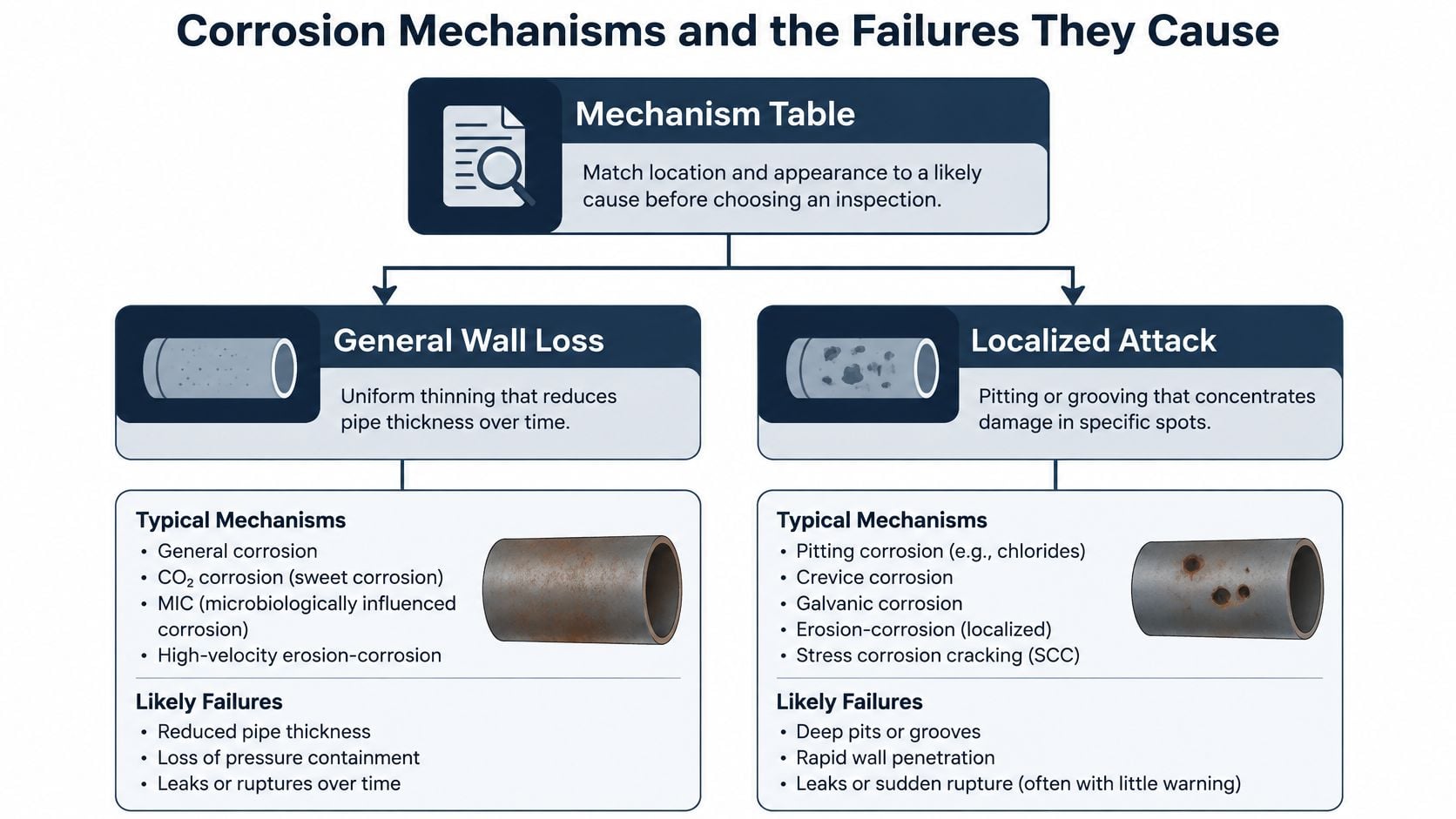
Corrosion Mechanisms and the Failures They Cause
| Mechanism | Where it appears | Visible signature | Typical failure |
|---|---|---|---|
| Uniform (general) corrosion | Wet carbon-steel lines, exposed external surfaces | Even scale and uniform thinning | Gradual loss toward t-min, leaks at the weakest point |
| Pitting | Stagnant water, low points, chloride brine | Isolated pits, often under deposits | Perforation with little change in average wall |
| Erosion-corrosion | Elbows, tees, reducers, high-velocity or two-phase flow | Grooved or smooth thinning downstream of turbulence | Sudden wall loss at fittings |
| CO2 (sweet) corrosion | Wet gas and water lines containing CO2 | Iron carbonate film, mesa-like attack | Rapid general or localized wall loss |
| H2S (sour) corrosion | Sour gas and crude lines with free water | Iron sulfide scale, blistering on inspection | Sulfide-film pitting, blistering, hydrogen-related cracking |
| Microbiologically influenced corrosion (MIC) | Water systems, dead legs, biofilm-covered sections | Tubercles over small pits | Local perforation at biofilm sites |
| Crevice or under-deposit corrosion | Flanges, gaskets, supports, deposits | Dark deposits, crevices at seals | Local attack hidden under the seal or deposit |
| Galvanic corrosion | Dissimilar metals joined in an electrolyte | Accelerated loss on the less noble metal near the joint | Rapid loss at the connection |
| Corrosion under insulation (CUI) | Insulated lines operating roughly 50-175 °C | Bulging or stained jacketing, wet insulation | Concealed wall loss found late |
| Water-driven dense-phase CO2 attack | Supercritical CO2 lines with free water | Localized attack at low points and injection points | Fast penetration once liquid water is present |
Two Families, Two Inspection Problems
General wall loss reduces thickness over a broad area. It is the easiest family to trend because repeat measurements at the same points usually show a consistent direction. It can still fail at a weld, thin area, or high-stress location, but the inspection logic is comparatively straightforward.
Localized attack concentrates loss in a pit, groove, crevice, or patch. Pitting produces narrow, deep holes. Under-deposit corrosion develops beneath scale, sand, sludge, or other material that holds corrosive water against the steel. Microbiologically influenced corrosion, or MIC, occurs where biofilms create local chemistry that accelerates attack, often beneath mounds called tubercles.
Other localized forms follow different clues. Galvanic corrosion occurs when dissimilar metals are electrically connected in a conductive liquid, with the less noble metal losing material near the joint. Erosion-corrosion combines chemical attack with flowing fluid, suspended solids, droplets, or turbulence that removes protective films. It's most suspicious downstream of elbows, tees, reducers, control valves, and injection points.
Consider a 150 mm crude line where chloride brine repeatedly collects at a low point. Readings on adjacent straight pipe remain acceptable, but a small cluster of pits deepens under deposit at the bottom. The eventual leak isn't evidence that thickness monitoring failed everywhere. It shows that the monitoring points missed the location where the governing mechanism operated.
Reading the Field Signature
Location often narrows the mechanism before detailed examination begins:
- Damage at the bottom of a horizontal run: Suspect water collection, under-deposit attack, or MIC.
- Thinning at an elbow extrados or downstream of a tee: Suspect erosion-corrosion and turbulence.
- Loss beside a flange, gasket, clamp, or support: Suspect a crevice or trapped moisture.
- Attack concentrated at a dissimilar-metal joint: Suspect galvanic coupling.
- Smooth, directional grooves: Suspect flow disturbance rather than stagnant-water pitting.
- Tubercles over pits: Sample the deposit and investigate microbial activity instead of treating it as ordinary scale.
A shortlist should come from two or three observed clues, not one isolated reading. Formal root cause failure analysis becomes important when the mechanism remains ambiguous, because inhibitor, metallurgy, drainage, and inspection choices all change with the diagnosis.
What Drives Internal Corrosion in Process Piping
A CO2 injection header running dry can jump to a much higher local corrosion rate after a dryer trip allows liquid water into a low section. In carbon-steel piping, persistent contact between the wall and an aqueous phase is often the controlling condition. The OSTI technical report on CO2 and H2S corrosion reports rates of several millimetres per year when carbon steel is directly exposed to water containing even moderate CO₂. Water presence, not gas composition alone, sets the corrosion rate when phases separate, condense, or become trapped.
Temperature, CO₂ and H₂S partial pressure, flow regime and velocity, water-phase pH, dissolved corrosion products, acetic acid, wetting behaviour, steel microstructure, and surface condition all affect the rate and pattern of attack. Small H₂S additions can change the protective-film behaviour: iron sulfide films form more readily than iron carbonate films. A film can limit general corrosion under one set of conditions, yet contribute to localized attack if it cracks, becomes uneven, or is stripped by flow.
Dense-Phase CO2 Shows the Water Effect Clearly
Dense-phase CO2 makes the role of water especially clear. A review of corrosion in dense-phase and supercritical CO₂ systems reports rates below 0.001 mm/year in dry CO₂ systems and above 0.1 mm/year, approaching 1 mm/year in some conditions, for water-saturated supercritical CO₂. It also contrasts approximately 0.4 mm/year in CO₂-rich conditions with about 20 mm/year in water-rich environments.
Use these reference rates to set the response, while checking the local damage pattern rather than relying on an average thickness:
- Dry dense-phase CO2 below 0.001 mm/year: Treat corrosion as negligible, but verify dehydration and water content continuously.
- CO2-rich conditions near 0.4 mm/year: Trend thickness at fixed grid points and investigate any upward shift.
- Water-saturated supercritical CO2 above 0.1 mm/year, approaching 1 mm/year: Shorten inspection intervals and review dryer, separator, and upset performance.
- Water-rich conditions near 20 mm/year: Treat the condition as critical and review shutdown and repair criteria under the plant's engineering authority.
After a dryer trip, liquid water may reach a low section, where localized metal loss can outpace the circuit average. Shortening inspection intervals alone leaves the cause unchanged. Check dryer alarms, separator levels, water-content analysers, inhibitor distribution if used, drain operation, and the duration of liquid-water exposure. A small number of acceptable thickness readings cannot rule out a governing pit at a water-collection point.
A rate increase after a process upset is process evidence first and an inspection-scheduling problem second.
Build a defensible trend by connecting free-water carryover, low-point and dead-leg behaviour, separator performance, pH, iron counts, inhibitor residuals, temperature, and velocity. Focus thickness readings on water-collection points, turbulent elbows and tees, injection quills, stagnant branches, and metal downstream of mixing or phase changes. Repeat readings at the same grid points and attach the relevant process history. Otherwise, a later reviewer cannot determine whether metal loss accelerated or the measurement location changed.
Inspection Techniques Compared and Where Each Fails
Four straight-run points all read above alert thickness on a 300 m water-injection line. That result describes those four locations, not the condition of the full line. A single pit can govern failure even when the average wall remains acceptable, so inspection plans need to target plausible damage locations and use enough measurements to support a remaining-life decision.
| Technique | What it detects | Blind spot | Best use |
|---|---|---|---|
| Spot UT thickness | Average wall at chosen points | Misses pits between readings | Trending at fixed, permanently marked points |
| UT grid or corrosion mapping | Wall-loss map across a defined area | Needs surface access and time | Localized damage in wet or deposit-prone service |
| Corrosion probes (ER or LPR) | Metal-loss rate at the probe location | Only measures at the probe; installation may require penetration | Tracking response to process upsets |
| Corrosion coupons | Mass loss over an exposure period | Needs weeks of exposure and insertion | Validating inhibitor and chemistry programs |
| Visual and borescope | Surface damage, deposits, internal condition | Cannot see concealed or thick-walled areas | Accessible sections, dead legs, low points |
| Guided-wave ultrasonics | Wall loss over long pipe runs from a few access points | Lower resolution; access limited near supports | Screening long runs before targeted UT |
| Pulsed eddy current | Wall loss through insulation or coating | Lower precision than direct UT | Screening for CUI |
| Thermography and moisture survey | Wet insulation and temperature anomalies | Indirect; does not measure wall loss | Prioritizing intrusive inspection |
| Iron counts and water chemistry | Process-driven corrosion activity | Not location-specific | Detecting upsets and water ingress early |
Why One Acceptable Average Can Mislead
The PHMSA presentation on internal corrosion monitoring limitations describes limits that matter when interpreting corrosion measurements: probes cover selected locations, their installation may require pressure-boundary penetration, and average wall-loss trends may not reveal incipient corrosion. It also reports 95% accuracy in its study setting for a dual-mode ultrasound and convolutional-neural-network method, while noting challenges when corrosion-particle concentrations are low.
Coupons require an exposure period. They help validate chemistry and inhibitor performance, but do not locate active damage. Electrical resistance and linear polarization probes respond faster, yet measure only at their installation points. Water chemistry can flag an upset, but cannot identify which elbow or low point is losing wall.
Direct measurement also depends on coverage. Spot ultrasonic testing, or UT, estimates remaining wall where the transducer contacts the pipe. A reading at one marked point cannot rule out a nearby pit. Guided-wave screening covers longer runs from fewer access points, but its lower resolution means indications need follow-up UT to determine their size. Pulsed eddy current screens through insulation, though precise remaining-life decisions require direct measurement.
Visual access has limits too. A camera can help find hidden drain problems with cameras, including deposits or obstructions. In process piping, internal visual inspection may require isolation, access, cleaning, and pressure-boundary controls. Those practical requirements affect whether a camera inspection is useful during an outage or routine work.
A Worked Coverage Example
A 60-point UT grid around the water-injection line's low point reveals a pit cluster where water and solids settle during reduced flow. The four straight-run readings remain above alert thickness, but they do not represent that location. The second survey examined the location where the failure mode was physically plausible.
Build coverage in stages:
- Screen broadly: Use guided-wave testing, chemistry, or operating history to identify suspect sections.
- Map locally: Apply a UT grid where water, deposits, turbulence, or screening indications concentrate.
- Trend continuously: Use probes or corrosion loops where process upsets can change the rate between outages.
- Verify chemistry: Use coupons, iron counts, pH, and inhibitor residuals to investigate why the rate changed.
Teams setting up this workflow can review ultrasonic testing maintenance applications alongside the limits of single-point thickness checks. Use fixed UT grids at risk points, probes for rate changes, screening for coverage, and chemistry to investigate cause. A defensible remaining-life decision depends on where readings were taken, how local damage is distributed, and whether the locations can be repeated consistently.
Corrosion Under Insulation Where to Inspect First
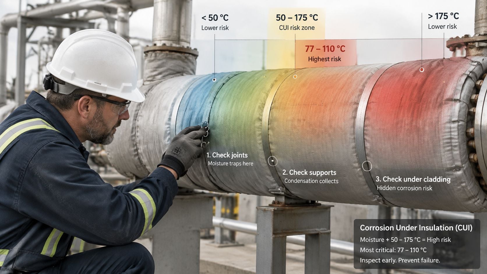
Temperature provides the first filter for corrosion under insulation, or CUI. The technical review of CUI fundamentals identifies approximately 50-175 °C as the risk range and an especially critical band around 77-110 °C. It estimates that CUI accounts for 40-60% of pipe-maintenance costs and about 10% of total annual maintenance costs in the referenced industries.
Removing insulation everywhere consumes outage labour and creates reinstatement risk. Leaving it in place makes ordinary visual inspection ineffective because the steel surface remains hidden. Ranking is therefore the control.
Ranking Sequence for Intrusive Inspection
- Temperature band: Place lines operating or cycling through the critical range first.
- Insulation condition: Prioritize wet, damaged, compressed, or missing insulation.
- Jacket and penetration defects: Inspect cracked seams, damaged flashing, unsealed supports, and instrument penetrations.
- Cycling and contaminants: Raise priority for temperature cycling, chloride exposure, and repeated wetting.
- Geometry and trapping points: Include dead legs, low points, clamps, and supports that retain water.
- Loss-of-containment consequence: Move hazardous, high-pressure, inaccessible, or shutdown-critical lines upward.
A 6-inch hot-oil return operating near 95 °C, cycling daily, and showing cracked jacketing at a support belongs near the top of the list. The support provides an entry point, cycling promotes wetting and drying, and the steel temperature sits in the sensitive band.
Thermography and pulsed eddy current are screening tools for deciding where to open insulation. They aren't proof that the concealed wall is acceptable.
Spot UT near supports, clamps, low points, and damaged jacketing can still miss the deepest patch. Screen first, open the highest-ranked windows, map the exposed area, then repair both metal and moisture barrier. Newer sensors also have limits, since many detect surface corrosion but can't reliably identify internal or buried defects, and long-term field validation remains limited.
Monitoring Strategies and Inspection Intervals
| Corrosion rate | Monitoring response | Reinspection interval |
|---|---|---|
| Below 0.05 mm/year | Routine grid and annual trend check | Up to 5 years or half remaining life, whichever is shorter |
| 0.05-0.13 mm/year | Add monitoring points and compare with process chemistry | 2-3 years, or half remaining life if shorter |
| 0.13-0.25 mm/year | Engineering review of process conditions and mechanism | Within 12 months |
| Above 0.25 mm/year | Root-cause review and repair or replacement plan | Within 3 months or per engineering review |
These are illustrative planning bands. The applicable piping code, jurisdiction, consequence class, damage morphology, and plant engineering basis determine the inspection interval. API 570 practice considers both short-term and long-term corrosion rates, generally using the higher rate for remaining-life and inspection decisions, subject to the code interval cap.
Calculating Remaining Life From Thickness Data
Use the measured wall thickness and corrosion rate to estimate remaining life:
Remaining life = (actual thickness − t-min) / corrosion rate
For a hypothetical 6-inch condensate line measured at 9.0 mm, with a t-min of 5.0 mm and a rate of 0.09 mm/year, the calculation is (9.0 – 5.0) / 0.09, or about 44 years. A 44-year projection still calls for reinspection in 2-3 years because the rate can shift with chemistry. Compare the next readings with process conditions, including condensate quality, oxygen ingress, flow, and operating temperature.
Average wall thickness can conceal the defect that fails first. If one pit is much deeper than surrounding metal, dividing average remaining wall by an average rate can overstate life. Use the deepest credible measurement, account for sizing uncertainty, and consider damage morphology in the engineering review.
Records Needed in the CMMS
Each circuit record should contain:
- Circuit ID and boundaries: Line identifiers, tied equipment, and isolation limits.
- Service and material: Fluid, phase, material specification, nominal thickness, and t-min.
- Inspection structure: Corrosion-loop ID and condition monitoring location, or CML, identifiers.
- Risk basis: Likely mechanism, consequence class, and special locations such as low points.
- Trend data: Latest short-term and long-term rates, remaining life, next due date, and linked work orders.
- Process context: Temperature, chemistry, upsets, inhibitor status, and water-ingress events.
Tag each stored reading to its constraint, fixed grid point, and operating condition so staff can reproduce the corrosion rate from the CMMS record. The guide to monitoring order processing bottlenecks offers a useful constraint-linked record concept for that data-tagging step. For piping, condition monitoring systems should connect readings to their fixed grid points and operating conditions. If stored data cannot reproduce a rate during an audit, that rate is not a defensible basis for a remaining-life decision.
Mitigation Options and When Each One Pays Off
| Option | Best for | Main limit | How to verify |
|---|---|---|---|
| Material upgrade (corrosion-resistant alloy or duplex stainless steel) | High-consequence sections with severe chemistry | Cost; weld and heat-affected-zone behavior needs its own plan | Positive material identification and weld inspection |
| Coatings and linings | External atmospheric exposure; internal lining of liquid lines | Holidays and damage; hidden CUI at breaks | Holiday testing and coating condition survey |
| Corrosion inhibitors | Wet carbon-steel gas and oil lines | Needs continuous injection and even distribution | Residual testing, coupons and probes |
| Cathodic protection | Buried or submerged steel | Needs electrical continuity and suitable electrolyte | Potential surveys against the -850 mV copper/copper-sulfate criterion used in common cathodic-protection criteria |
| Hydraulic controls (velocity limits, dead-leg removal, drainage, separation) | Erosion-corrosion and water accumulation | Throughput or process-change constraints | Flow review and low-point checks |
| Dehydration (CO2 and wet gas) | Dense-phase CO2 and wet gas service | Dryer reliability and upset response | Dew-point or water-content monitoring with alarms |
Decision Order
Choose mitigation by failure consequence first, then process severity, maintenance access, and whether damage is general or localized. This prioritization avoids paying for resistant metallurgy when geometry is trapping water. Average wall thickness alone is not enough: a single deep pit can govern failure, so retain targeted inspection at the locations most likely to hold water or deposits.
Inhibitors can pay off in wet carbon-steel gas and crude lines when injection is continuous, reaches the water-wetted wall, and residuals are tested. Batch treatment without residual confirmation provides weak assurance. Use probes and coupons to check whether the chemistry change reduced metal loss.
Cathodic protection suits buried or submerged steel. Its performance depends on electrical continuity, coating condition, electrolyte contact, and periodic potential surveys. Apply it to external corrosion; it does not control internal process corrosion.
Material upgrades make sense where consequences are high, chemistry is severe, inspection access is poor, or repeated carbon-steel repairs cost more than replacement. Corrosion-resistant alloys and duplex stainless steels still require weld procedure control, positive material identification, and inspection of welds and heat-affected zones. Match the alloy to chlorides, H2S, temperature, and cracking risks, not just general metal loss.
Coatings and linings act as barriers, but holidays, impact damage, poor surface preparation, and trapped moisture can expose local areas. Damaged insulation can conceal external attack, so plan inspection windows. Holiday testing locates discontinuities; recurring condition surveys check whether field damage has exposed the steel again.
Hydraulic correction often delivers the best return, as beside a capped branch where water pools. Removing the dead leg, adding a drain, and improving separation address the cause directly. An alloy spool may tolerate pooled water longer, but it leaves stagnant inventory and deposit risk in place.
Pipe replacement can also be practical outside process service, as with Stultz Plumbing repiping services for building piping. Industrial replacement has a different threshold: pressure, hazardous inventory, outage scope, and code documentation shape the decision. A structured FMEA for manufacturing helps compare options by failure mode, detectability, and consequence rather than purchase price alone.
Confirm Your Corrosion Circuits Before Your Next Turnaround
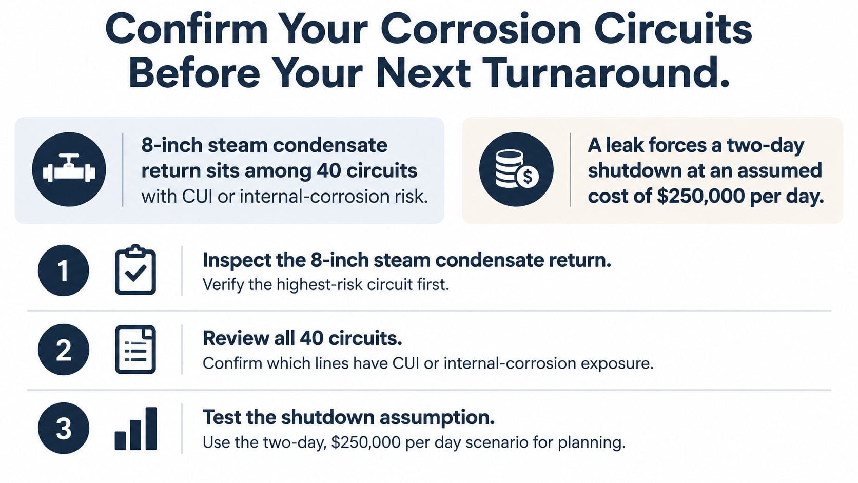
An 8-inch steam condensate return may sit among 40 circuits with CUI or internal-corrosion risk, yet only a few can receive intrusive inspection during the next turnaround. A worked example needs its assumptions stated clearly. If a leak forces a two-day shutdown at an assumed US$80,000 per day, one event costs an assumed US$160,000 before repair materials, cleanup, and restart losses. A targeted UT grid and CUI screening on that circuit costs a fraction of the assumed event, so it can pay back through one avoided failure.
The wider economics point in the same direction. The NACE International IMPACT study estimated global corrosion cost at approximately US$2.5 trillion in 2013, equivalent to about 3.4% of global gross domestic product, and concluded that established practices could reduce damage by roughly 15-35%.
Six Actions Before the Scope Freezes
- List every circuit: Assign a consequence class based on fluid, pressure, location, and shutdown effect.
- Assign the likely mechanism: Use service, geometry, temperature, deposits, and past damage signatures.
- Baseline the fixed grid: Measure the points where water, turbulence, insulation damage, or stagnation concentrates loss.
- Add rate trending where needed: Install probes or define corrosion loops for circuits sensitive to process upsets.
- Set and record intervals: Apply the plant's code basis and rate bands, then tag each circuit and CML in the CMMS.
- Review every rate change: Compare metal loss with chemistry, water ingress, velocity, temperature, and inhibitor records before extending or shortening an interval.
Forge Reliability offers a free reliability assessment that can rank corrosion circuits, test inspection coverage, and set monitoring priorities before the next shutdown.
Request a free reliability assessment from Forge Reliability to rank pipe corrosion circuits by consequence, identify inspection blind spots at low points, fittings, and insulated sections, and set defensible monitoring intervals before the next turnaround.