
A new pump train has been running for nine days and the mechanical seal is already leaking. Down the line, a motor that has run for years trips for no obvious age related reason, while a gearbox nearby shows rising metal in its oil. A planner who treats all three events the same way will waste money on at least two of them. The bathtub curve failure rate helps sort those events, but only if the team sorts by failure mode, not by calendar age alone.
That distinction is the work of a reliability program. Each failure mode sits in a phase, and the phase points to a response. One mode needs a commissioning fix, another needs monitoring, and another may justify planned replacement.
Table of Contents
- Bathtub Curve Failure Rate by Life Phase
- How the Three Phases of the Curve Form
- Calculating Failure Rate, MTBF and Weibull Shape
- Early-Life Failures During Commissioning
- Random Failures and the Constant Rate Model
- Wear-Out Failures and Age-Based Replacement
- Build an Asset Phase Register
Bathtub Curve Failure Rate by Life Phase
A maintenance manager doesn't need a calculation to make the first sorting decision. The table below puts the bathtub curve failure rate into plant terms, pairing each phase with its trend, its likely causes, and the response that fits.
| Phase | Failure rate trend (Weibull β) | Typical duration | Typical plant causes | Maintenance response |
|---|---|---|---|---|
| Early life (infant mortality) | Decreasing (β below 1) | Weeks to a few months | Assembly errors, contamination, wiring faults, seal leaks at commissioning | Acceptance testing and root-cause correction |
| Useful life | Approximately constant (β near 1) | Most of the operating life | Overloads, electrical transients, contamination, random component faults | Condition monitoring, corrective repair, failure-finding |
| Wear-out | Increasing (β above 1) | Late life, as degradation accelerates | Fatigue, corrosion, erosion, lubricant breakdown, seal wear | Overhaul, redesign or age-based replacement where data support it |
How to place a failure mode in a row
Start with the failure history for one mode, not for the whole asset. A centrifugal pump can have seal leaks that cluster in the first weeks after a rebuild, starter faults that occur at any age, and bearing wear that rises late in life. Those are three different rows, even though they share one asset tag.
Planners should ask when the failures occur relative to installation, overhaul, or exposure hours. If failures fall quickly after startup and then stop, the mode belongs in early life. If they spread across operating time without an age pattern, useful life is the better fit. If they concentrate at higher ages and condition data worsen with them, wear-out becomes credible.
Why one policy fails
A fixed replacement interval helps only the third row, and only when the data support it. Applied to early-life defects, replacement reinstalls the same assembly error. Applied to random faults, it discards healthy life and can introduce new installation defects. Applied too late to true wear-out, it misses the window for a planned outage.
Sorting rule: Establish the phase for each failure mode first, then take the response from that row.
The practical takeaway is simple. One maintenance policy can't serve all three phases at once. Teams that keep that rule visible in planning meetings stop debating asset age in the abstract and start debating evidence for a specific mode.
How the Three Phases of the Curve Form
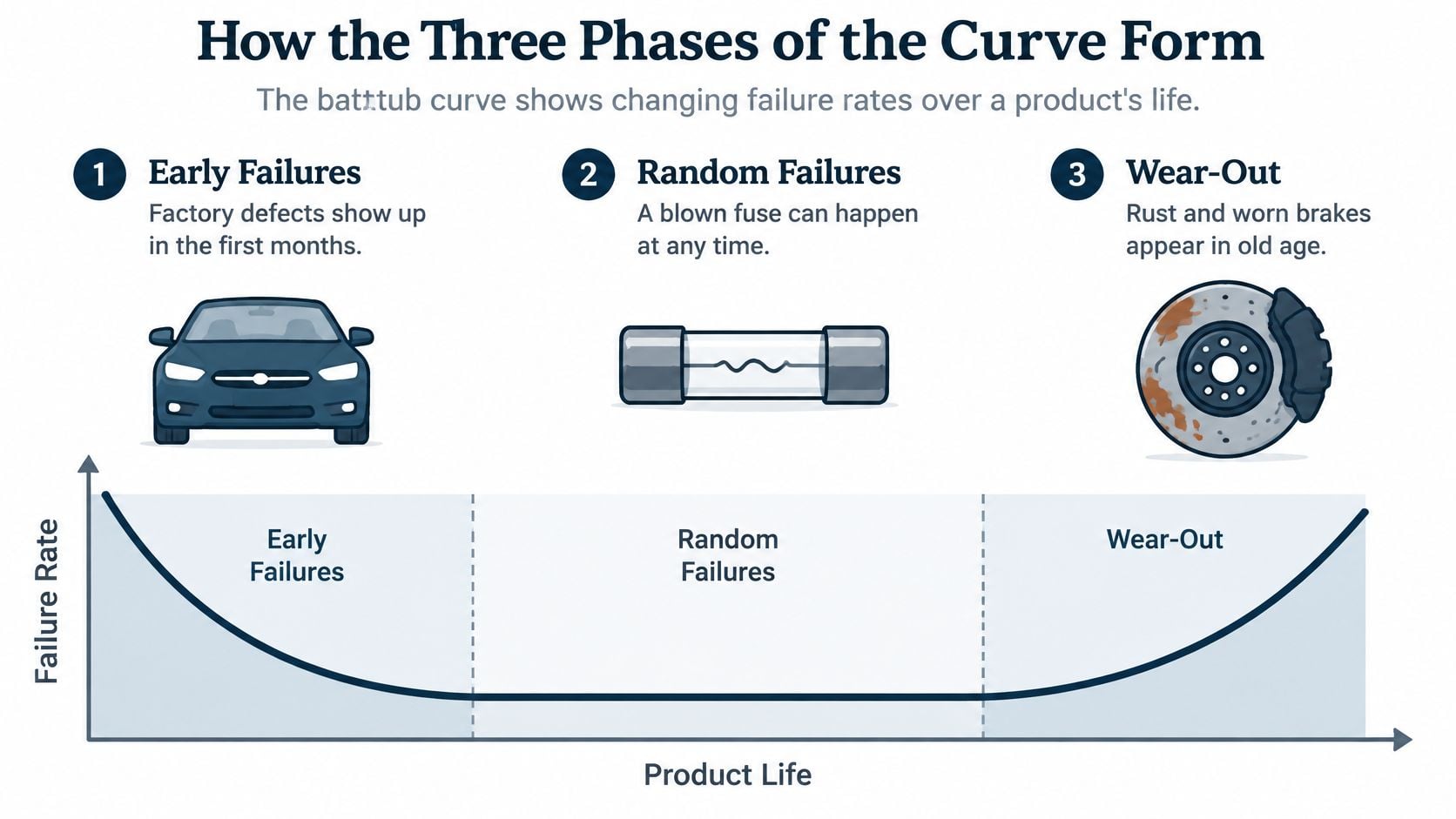
A new car offers a useful analogy. Factory defects, a loose connector, or a misaligned panel tend to show up in the first months. After those problems are corrected, a blown fuse or a punctured tire can happen at almost any time. Rust, worn brakes, and tired suspension parts arrive much later, after years of exposure and use.
Industrial equipment follows a similar population pattern for mechanical reasons. The instantaneous failure rate, also called the hazard rate, is the chance that a unit that has survived to a given age fails in the next interval. That conditional idea matters. It is not the share of the original population that has failed, and it isn't a promise about one machine.
Why the shape bends
The NIST handbook on the bathtub curve describes an early-failure period with a high but rapidly declining rate, a useful-life period with an approximately constant intrinsic failure rate, and a wear-out period in which the rate increases as materials degrade.
Weak units explain the first drop. A pump with piping strain, a motor with a damaged lead, or a gearbox filled with contaminated oil fails sooner than its peers. Once those weak units are repaired or removed, the surviving population looks stronger, so the population rate falls even if no individual machine improves.
The flat middle follows because the remaining causes don't respect age. Process upsets, voltage events, foreign material, and occasional component faults strike survivors at a roughly steady conditional rate. Late in life, fatigue cracks grow, insulation embrittles, lubricant breaks down, and seals wear. Those aging mechanisms accumulate, so the conditional risk rises.
The curve describes a population's failure rate, not a guaranteed life for any single asset.
A practical test keeps the analogy honest. For a pump, motor, or gearbox, the team should ask whether failures cluster near installation, spread across operating time, or rise with age. The answer, supported by failure ages and condition evidence, determines which phase best describes that failure mode.
Calculating Failure Rate, MTBF and Weibull Shape
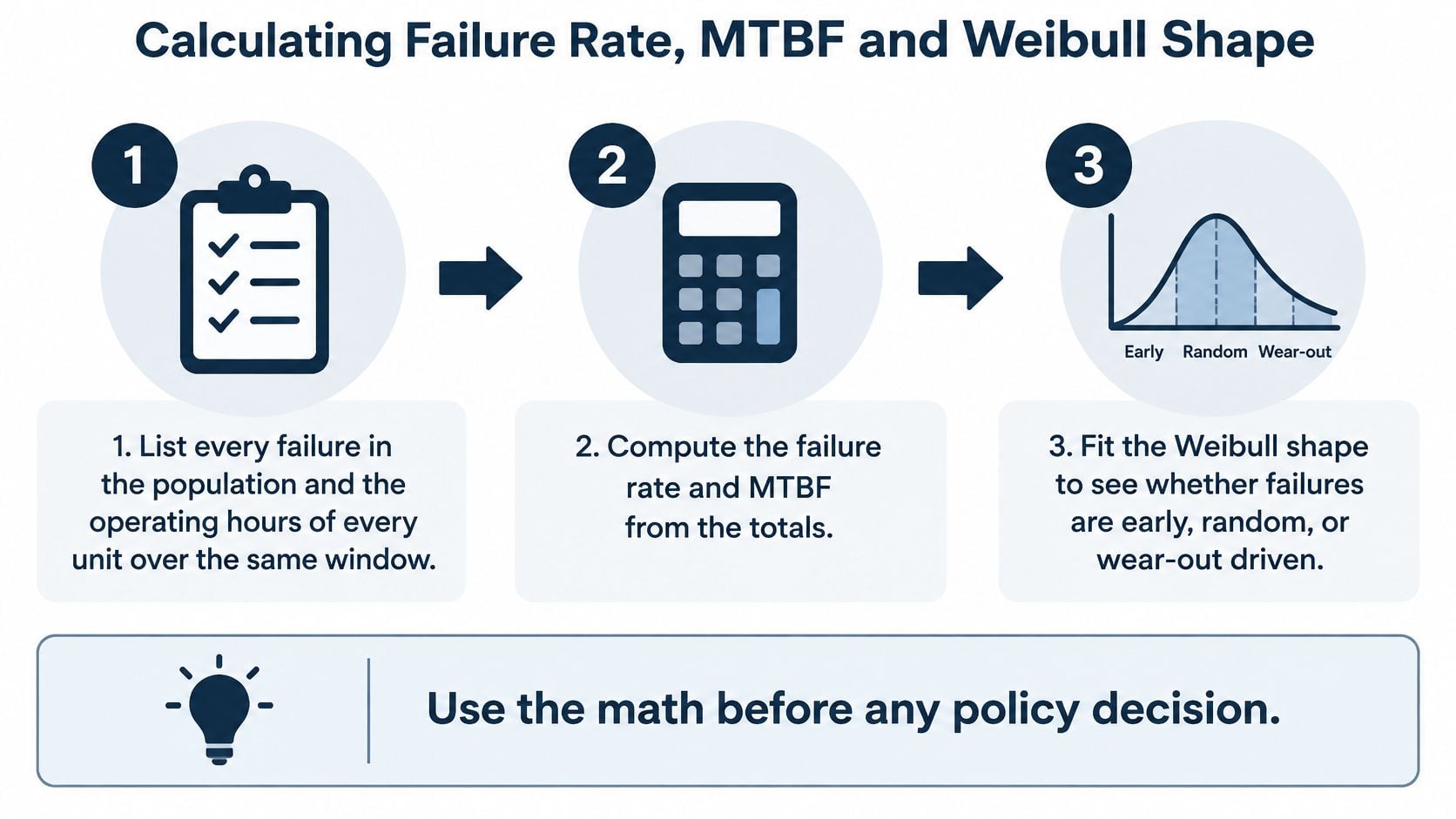
Policy debates go better after the arithmetic is visible. The routine below gives planners a repeatable way to estimate the bathtub curve failure rate and test whether a single average is defensible.
A five-step routine
- Collect the population record: List every failure and the operating hours of every unit over the same window.
- Compute the failure rate λ: Divide failures by total operating hours.
- Compute MTBF: Divide total operating hours by failures, and use it as a rate summary only if the rate is approximately constant.
- Fit a Weibull distribution: Plot failure ages, read the shape parameter β, and classify decreasing, constant, or increasing behavior.
- Check confidence bounds: Treat estimates from a few failures as wide ranges, not precise limits.
| Quantity | Formula or method |
|---|---|
| Failure rate λ | 6 failures / 96,000 hours = 0.0000625 per hour, or 62.5 per million hours |
| MTBF | 96,000 hours / 6 failures = 16,000 hours |
| Confidence bounds | Chi-square bounds on failure count and operating hours; wide with only 6 failures |
| Weibull shape β | Slope of the Weibull probability plot of failure ages; below 1 decreasing, near 1 constant, above 1 increasing |
| Characteristic life η | Age at which 63.2% of the population has failed |
Worked pump example
Say 12 centrifugal pumps each run 8,000 hours, for 96,000 operating hours, and the population records 6 failures. The failure rate is 6 divided by 96,000, which gives 62.5 failures per million hours. The corresponding MTBF is 16,000 hours. A planner can use the detailed mean time between failure calculation to check that reciprocal relationship, but the number still needs a phase test.
Suppose the six failures aren't one mode. Seal leaks occur soon after commissioning, starter faults spread across ages, and bearing failures occur at older ages. If bearing failure ages produce β of 2.8, the bearing mode has an increasing hazard. MTBF then stops being a useful guide for that mode, because risk at low age isn't the same as risk at high age. The planner should use the Weibull fit to set an inspection or replacement age where conditional risk becomes unacceptable.
Units still running at the end of the window count as suspensions, not failures. Their hours carry information because they survived to that age. Ignoring them makes life look shorter than it is.
Sparse data need restraint. A Weibull fit on very few failures isn't reliable, and confidence bounds will show that uncertainty. For failure modes where time-based tasks are considered, Forge Reliability conducts age exploration using facility failure history, published databases such as OREDA and IEEE 493 (Gold Book), and Weibull analysis where sufficient data exists. That hierarchy keeps plant evidence first while giving sparse populations a checked reference point.
Early-Life Failures During Commissioning
A newly commissioned centrifugal pump train makes early-life behavior easy to see. Seal leaks appear during the first runs, coupling alignment shifts after grouting cures, and a loose motor termination heats under load. None of those events proves the pump has worn out. Each one points back to manufacture, transport, installation, or startup control.
The correct response is inspection and correction while the evidence is fresh. Replacement without diagnosis can return the same defect to service, especially when piping strain or contaminated flush fluid caused the first leak.
Commissioning checks that catch defects
- Record baselines: Capture a vibration spectrum and motor current at the normal operating point.
- Verify alignment twice: Check laser alignment after grouting and again after the first thermal run.
- Protect the seal: Verify seal flush flow and check piping strain on the pump casing.
- Check electrical integrity: Torque-check terminations and confirm phase balance.
- Clean the lubrication system: Flush the system and sample oil for debris before sustained operation.
Those checks create a reference for later trending. A baseline spectrum taken at a known speed, load, and temperature lets an analyst separate a startup defect from later degradation. An early oil sample does the same for wear debris and contamination.
When a repeat failure changes the task
A repeat failure at the same location inside the early window shouldn't trigger a shorter replacement interval. It should trigger root-cause analysis using 5-Why or fault tree methods. The question changes from which part failed to which process allowed the defect. A structured FMEA for manufacturing review helps the team connect the failure mode to installation controls, spare quality, and acceptance criteria.
Common mistakes keep early-life problems alive:
- Replacing parts at three months: Crews change seals or bearings without identifying strain, contamination, or misalignment.
- Ignoring first oil samples: Debris in early samples gets dismissed as normal break-in material.
- Treating warranty returns as wear: A returned component closes commercially while the plant defect remains open technically.
Clustered early failures mean the producing process must be fixed and closure must be tracked. The stable period shouldn't be declared until corrective action is verified under operating conditions.
Random Failures and the Constant Rate Model
A food plant with 200 motors and variable-frequency drives, or VFDs, gives the constant-rate model a fair test. Some drives trip after power events, some motors fail after cooling paths foul, and some starters fail without a clear age pattern. Planners still need forecasts for spares and crew hours, even though individual failure dates remain uncertain.
The NIST guidance on constant failure rate models treats this region with an exponential or homogeneous Poisson-process approach because many systems spend most of useful life in the approximately flat region. Under that model, MTBF estimates and confidence bounds can be calculated from operating and repair data. The estimate supports fleet planning. It doesn't prove that a particular motor will fail at its MTBF.

Test the model before using it
Engineers should plot failures against age and separate causes first. Commissioning defects, overloads from process upsets, thermal cycling, power-quality events, and genuine wear-out shouldn't be blended into one rate. If β stays near 1 and failures spread across ages, the constant model fits well enough for fleet estimates. If failures cluster in age brackets, it doesn't.
A constant rate also doesn't mean failures arrive evenly. A fleet can record none for months and then several close together. That's compatible with random timing. Planners who expect one failure every MTBF interval will misread normal clustering as a sudden program failure.
A steady failure rate is a reason to monitor the asset, not a reason to replace it on a calendar.
Actions that fit random failures
Useful actions expose stress or detect hidden failure. Motor current signature analysis can reveal electrical and load related anomalies, thermography finds hot connections and cooling problems, and function testing confirms that starters and protective devices still operate. Power-quality logging links trips to transients, while cooling-path inspection removes a common thermal stressor. A disciplined condition-based maintenance program ties those readings to corrective repair and root-cause follow-up.
One warning overrides the model. Rising vibration, temperature, oil debris, or leakage means the asset no longer behaves like a constant-rate population. At that point, a degradation model or Weibull analysis fits better than a fleet average.
Wear-Out Failures and Age-Based Replacement
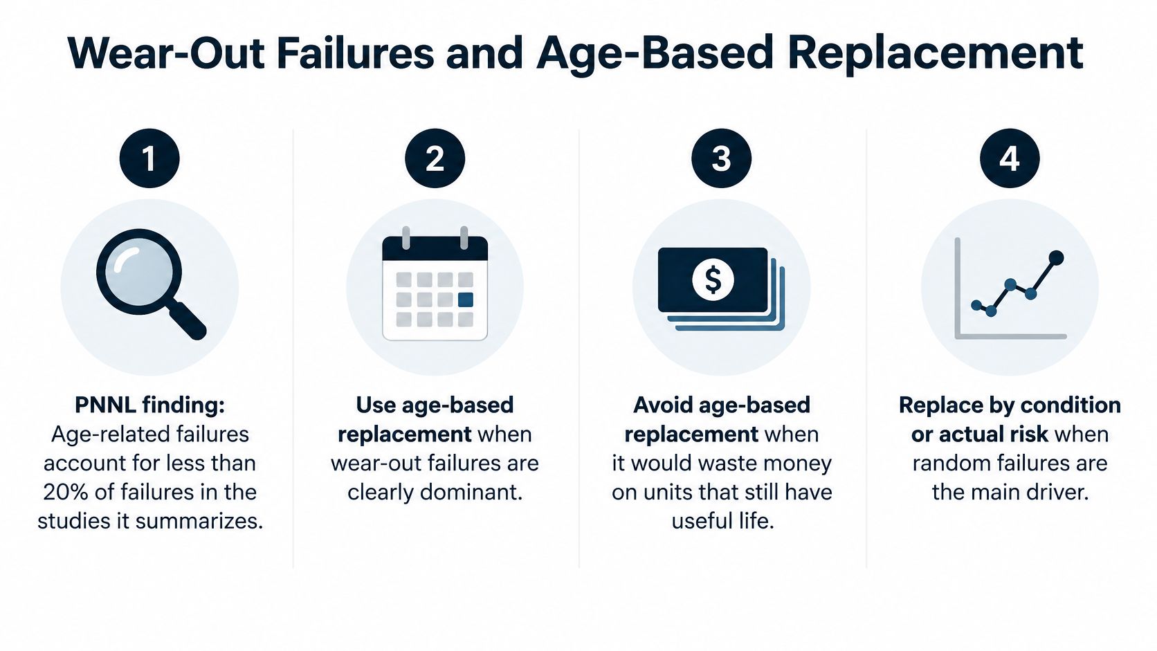
Age-based replacement sounds decisive, but it only works when failure risk rises with age and the task intervenes before functional failure. The Pacific Northwest National Laboratory summary of reliability centered maintenance studies reports that age-related failures account for less than 20% of failures, while random failures account for roughly 80%, in the studies it summarizes. Those shares aren't a universal rule for every component. They are a warning against blanket replacement.
Decision sequence
A planner should confirm β above 1 from failure history for the specific mode. Next, the team identifies the physical mechanism, checks whether a condition indicator detects it with enough warning, and compares task cost with failure consequence. If failure data don't support an increasing hazard rate with age, Forge Reliability determines time-based tasks are not applicable regardless of manufacturer recommendations or historical practice.
That discipline matters in machining areas as well as rotating equipment. Tool wear can be age related, but operators still need operating limits and inspection evidence. The resource on cutting speed limits for carbide tools is useful context for how process limits interact with tool degradation, rather than assuming hours alone define tool life.
| Failure mode | Expected phase | Detection method | Task |
|---|---|---|---|
| Pump bearing wear | Wear-out | Vibration bearing-defect frequencies, oil debris | Lubrication control and planned replacement at inspection |
| Motor insulation aging | Wear-out | Insulation resistance, polarization index, thermography | Rewind or replace on a degrading trend |
| VFD electrolytic capacitor aging | Wear-out | Capacitance and ripple tracking, temperature | Replace on verified age and trend |
| Gear tooth fatigue | Wear-out | Vibration, ferrography | Overhaul when defect growth is confirmed |
| Motor starter contact failure | Random | Thermography, contact resistance, function testing | Function testing and failure-finding, no age limit |
| Seal leakage | Mixed | Leakage monitoring, seal flush pressure | Seal flush optimization and condition-based repair |
Match the task to the mechanism
Pump bearing wear often gives warning through defect frequencies and debris, so planned replacement at inspection can beat a blind age limit. Motor insulation aging needs trendable electrical tests. A single insulation resistance reading invites argument, while a falling polarization index with rising temperature supports rewind planning.
VFD capacitors present a narrower case for age involvement because electrolyte degradation advances with time and temperature. Even there, capacitance, ripple, and thermal evidence should verify the age claim. Gear tooth fatigue needs confirmed defect growth before overhaul, since opening a gearbox carries its own installation risk.
Random contactor failure belongs in a different decision bucket. Function testing and failure-finding expose hidden faults without discarding serviceable contacts. Seal leakage is mixed, so flush pressure, face condition, and leakage trend should separate commissioning defects from face wear.
Where no effective task exists, redesign or run-to-failure can be rational. Redesign fits high-consequence modes with a correctable stressor, such as poor seal flush or chronic overload. Run-to-failure fits low-consequence modes where monitoring or scheduled work costs more than the failure. A remaining useful life estimate helps only when degradation is measurable and the failure definition is clear. Without those conditions, a precise life number gives false confidence.
Build an Asset Phase Register
An asset phase register turns phase sorting into a Monday-morning deliverable. It holds one row per failure mode on critical equipment, with columns for asset tag, failure mode, failure count and operating hours, β with its phase label, the selected response, and the review date. A planner can maintain it beside the criticality list instead of a separate reliability report.
The habit that makes the register work is sorting modes, not assets. One gearbox can carry three rows in three different phases, and the phase on each row, not the gearbox's age, decides the response.
Gearbox set example
Consider eight gearboxes driving induced-draft fans on a shared duty cycle. Gear tooth pitting across the population fits β of 2.4, so that row sits in wear-out and its replacement interval comes from the Weibull fit and inspection findings. Output-shaft seal weeps clustered in the first months after the last rebuild fit β below 1, so that row stays in early life until the installation root cause is verified. Lube pressure-switch faults fit β near 1, so that row goes to function testing rather than age replacement.
Each row forces a different owner conversation. Operations owns overload evidence, maintenance owns rebuild quality, and reliability owns the fit and the phase call. That separation keeps one average gearbox MTBF from hiding three different decisions.
Keep nominal age from overruling evidence
The NASA analysis of 104 orbital missions launched from 1960 through 1980 reports that more than two-thirds of analyzed systems show infant mortality followed by a constant failure rate with no identifiable end-of-life aging period, and that by the 1970 to 1974 period wear-out lives had broadened enough that failures no longer formed a concentrated cluster.
Plant teams should apply that caution directly. Before any replacement interval changes, Weibull analysis, failure-mode review, and condition indicators should confirm wear-out. A governed CMMS asset management record keeps operating hours, failure codes, and review dates consistent enough for that test. Review each register row after 12 months of new data, and move any row whose β has crossed into a different phase.
Request a free reliability assessment from Forge Reliability to build the register. The assessment maps critical equipment to these phases, tests failure histories with Weibull analysis, and separates assets that need condition monitoring from those with defensible age-based tasks.