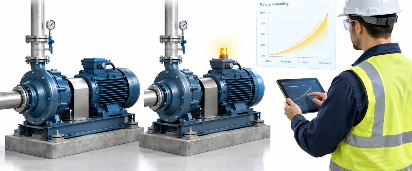
A maintenance planner is looking at two centrifugal pumps with identical nameplates, identical service, and apparently identical maintenance histories. Operations wants both treated the same. The vibration analyst knows one pump is stable, while the other has rising bearing vibration, a recent alignment correction, and an inspection already pushed beyond its original window. A single probability of failure assigned to both assets would simplify the spreadsheet, but it would also hide the decision that matters: which pump needs work first, and how soon?
Probability of failure becomes useful only when it changes that decision. It must be tied to a named failure mode, a defined time window, current operating conditions, available inspection capacity, and the consequence of getting the call wrong. The practical question isn't whether a model produces a number. It's whether the number creates a defensible work order before the failure creates an unplanned outage.
Table of Contents
- What Probability of Failure Actually Means on a Plant Floor
- The Math Behind Probability of Failure
- Weibull and Exponential Models in Practice
- Data Sources and How to Estimate Probability of Failure
- Worked Examples for Pumps, Motors, and Compressors
- How Probability of Failure Fits Into RBI and FMEA
- Limitations and Common Mistakes to Avoid
- Validating Probability Estimates and Next Steps
What Probability of Failure Actually Means on a Plant Floor
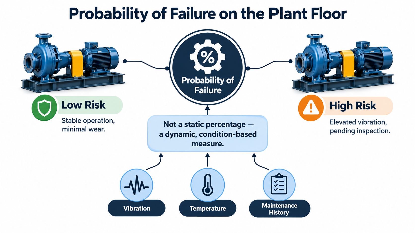
The planner can reasonably ask why the two pumps should receive different treatment. Their nameplates may match, but probability of failure isn't stamped permanently onto an asset. It is an estimate that changes as the pump ages, its load shifts, condition indicators move, and maintenance findings add evidence.
The National Institute of Standards and Technology describes the bathtub curve as a foundational model for the probability of failure over an asset's life. It contains an early-failure period, a useful-life period with an approximately constant failure rate, and a wear-out period in which failure rate rises as materials degrade and components approach their physical limits (NIST's explanation of the bathtub curve).
The estimate must answer a decision
For the stable pump, a low current risk band may support continued operation with routine route-based vibration collection. For the pump with high vibration, the same nominal fleet estimate could be reckless because its asset state has changed. If the pump serves a single production train with no practical standby, the intervention threshold should also be lower than it would be for a small auxiliary pump whose failure can be isolated without production impact.
A plant-floor probability statement should therefore include:
- Failure mode: bearing defect, seal leakage, impeller erosion, insulation breakdown, or another specific mechanism.
- Time window: the next operating period, inspection interval, or planned outage window.
- Evidence: vibration trend, oil debris, thermal pattern, motor current, work history, and operating load.
- Consequence: safety, environmental, production, equipment, and repair implications.
- Action threshold: continue running, inspect, create a planned work order, or remove from service.
Practical rule: A probability estimate that doesn't change inspection timing, work priority, or operating control is usually reporting, not reliability engineering.
The distinction is especially important for teams communicating reliability decisions outside engineering. A concise practical guide for ecommerce engineering teams also helps explain why reliability work depends on failure mechanisms, operating context, and repeatable engineering decisions rather than a headline metric.
The plant can use an equipment failure patterns reference to connect the statistical estimate to the asset's actual life pattern. The working standard remains simple: estimate risk for the right failure mode, over the right interval, then assign an action that someone can execute.
The Math Behind Probability of Failure
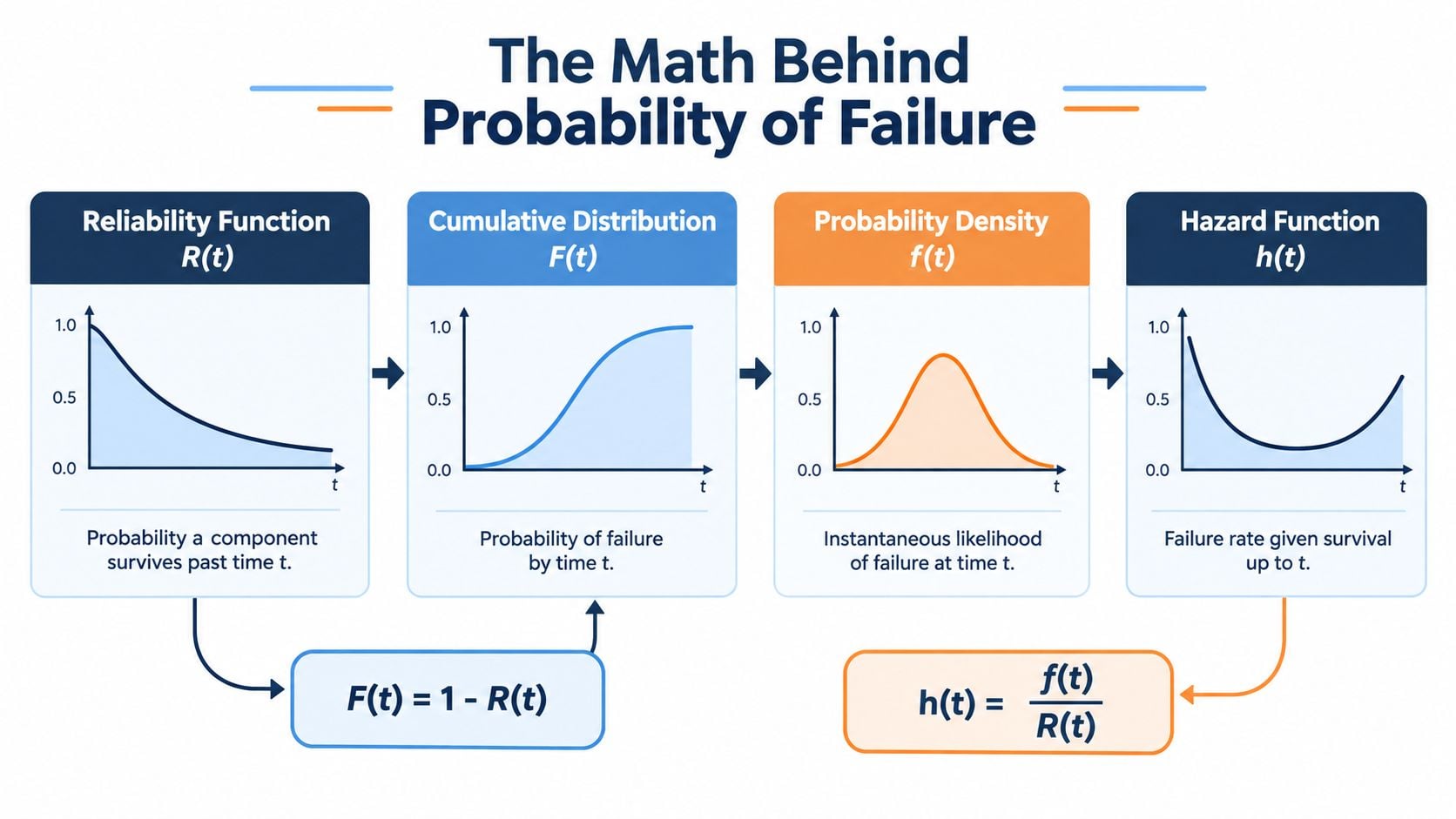
Probability of failure is easier to use once the related functions are separated. Each answers a different question about a population of similar components or about an individual asset represented by a statistical model.
Four functions, four questions
The reliability function, written as R(t), means the probability that an item survives beyond time t. If a bearing population has R(t) equal to a certain value at a selected runtime, that value describes survival past that runtime, not the likelihood of failure during every future period.
The cumulative distribution function, F(t), means the probability that failure has occurred by time t. The relationship is:
F(t) = 1 – R(t)
The probability density function, f(t), describes how failures are distributed around time t. It is not, by itself, the probability that one asset will fail in a maintenance window. It shows where failures are concentrated across the modeled population.
The hazard function, h(t), is the instantaneous failure rate conditional on survival up to t. In plain language, take the components still operating at a particular moment and examine the rate at which those survivors are failing at that moment:
h(t) = f(t) / R(t)
A constant hazard rate doesn't mean a constant probability of failure over a year. It means the conditional rate remains stable as time advances under the model assumptions. The actual probability over a selected interval still depends on the length of that interval and the survival distribution.
Choose the window before reading the result
A planner should never receive “the pump has a probability of failure of X” without a time horizon. The relevant question might be whether the pump will fail before the next inspection, before the next scheduled outage, or during the operating period that cannot be interrupted.
That window also determines the maintenance response. A moderate short-window risk may justify a targeted inspection if the failure consequence is limited. The same estimate can justify immediate intervention when the pump protects a hazardous process or has no installed standby.
The bathtub curve reinforces the point. Early failures may reflect manufacturing, installation, commissioning, or design weaknesses. During useful life, random failures can dominate. During wear-out, degradation changes the hazard. The maintenance strategy must follow the phase rather than treating probability of failure as one fixed percentage. Engineers needing a quick reference for fleet reliability definitions can use this mean time between failures calculation guide, but MTBF alone shouldn't replace a time-bounded failure estimate.
Weibull and Exponential Models in Practice
The Weibull distribution is often the most practical life-data model for plant equipment because its shape parameter, β, describes how the failure rate changes with time, while its scale parameter, η, represents characteristic life within the fitted population.
For a centrifugal pump impeller or bearing population, the shape interpretation is operationally useful:
- β less than 1 indicates a declining failure rate, commonly associated with infant mortality, installation defects, or commissioning problems.
- β approximately equal to 1 indicates an approximately constant failure rate, consistent with random failures during useful life.
- β greater than 1 indicates an increasing failure rate, consistent with aging, wear, fatigue, or degradation.
Suppose a plant fits life data for identical pump bearings and finds evidence consistent with β greater than 1. The result doesn't automatically authorize replacement of every bearing at the same age. It says the population is showing an aging pattern, which supports closer condition monitoring, inspection planning, and an economic comparison between planned replacement and run-to-failure.
Match the model to the question
The exponential model assumes a constant hazard. It can be defensible when the equipment has no clear wear-out mechanism, when failures are approximately random, or when the available data cannot support a more complex model. Electronics and complex systems with no identifiable age-related pattern may fit this logic better than a pump bearing exposed to lubrication contamination and alignment forces.
Weibull is more useful when the plant needs to distinguish early-life defects from aging. It can answer whether failure risk is rising with runtime, while the exponential model mainly answers how a constant-rate population behaves over a selected interval.
A Weibull probability plot deserves cautious reading. A roughly linear pattern may support the model over the observed range, but scatter, mixed failure modes, maintenance interventions, and changing duty can distort the fit. Two parameters are often enough for a plant decision. Adding parameters without enough evidence can fit noise rather than improve the work plan.
A reliability team evaluating Weibull analysis software should require transparent assumptions, treatment of suspended items, confidence bounds, and outputs that planners can use. A complex curve that cannot produce an inspection interval or replacement rule is academic theater.
Data Sources and How to Estimate Probability of Failure
The model is only as credible as the evidence underneath it. A plant usually has more data than it realizes, but the records rarely arrive in a form that can be fitted immediately.
Build the evidence base
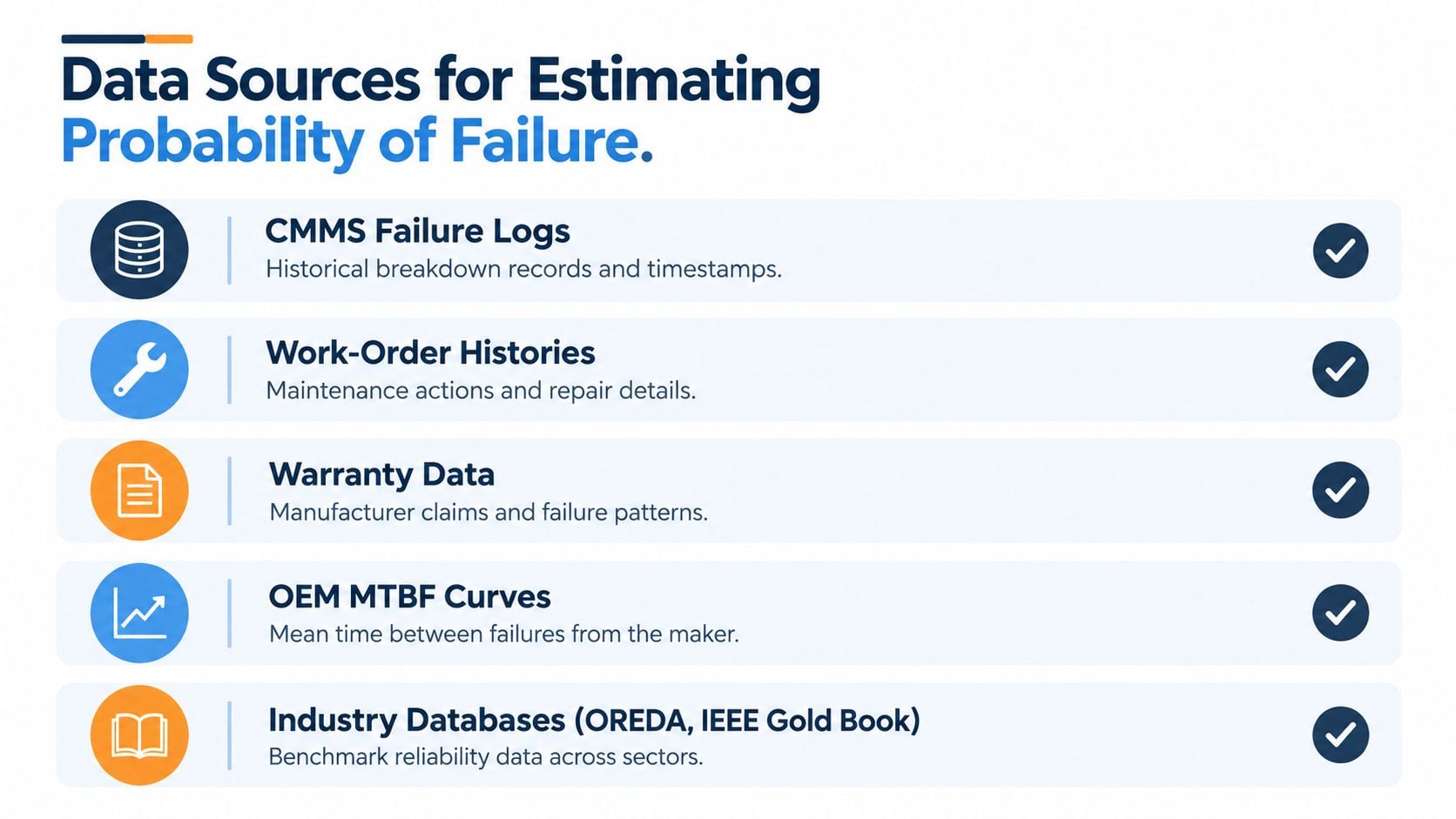
The most useful sources include:
- CMMS failure logs: Breakdown dates, asset identifiers, failure codes, and restoration times provide the foundation, but technicians may record similar mechanisms under different labels.
- Work-order histories: Corrective actions, inspection findings, replaced parts, and operating observations reveal degradation that never became a full failure.
- Warranty data: Manufacturer claims can expose recurring defects, although warranty populations may differ from the plant's duty cycle.
- OEM MTBF curves: These provide a starting benchmark, not a plant-specific truth. Duty, contamination, loading, installation quality, and maintenance practice can shift actual behavior.
- Industry databases: OREDA and the IEEE Gold Book can support comparative reasoning, but fleet heterogeneity must be stated explicitly.
- Condition-monitoring trends: Vibration, oil analysis, thermography, ultrasound, and motor-current data can show changing condition before a breakdown, provided measurements are repeatable and linked to failure modes.
Fit the model without hiding uncertainty
A small CMMS export might contain several failed pump bearings, several pumps still operating, and assets removed from service for reasons unrelated to bearing failure. The surviving and removed assets are censored observations, meaning their complete failure life isn't known. Excluding them biases the estimate toward the failures that happened to be observed.
A defensible workflow looks like this:
- Standardize asset identity, failure mode, runtime basis, and intervention date.
- Separate bearing failure from seal, coupling, impeller, and process-induced events.
- Record operating regime, including speed, load, fluid, temperature, and contamination exposure.
- Include surviving assets and mark their observation as censored.
- Fit β and η using a method appropriate to the sample and censoring pattern.
- Report confidence intervals around both parameters instead of presenting only point estimates.
- Backtest the resulting probability bands against later failures and inspection findings.
A model based on a few clean failures may still be useful for triage, but it shouldn't be presented as a precise plant law. Missing near-misses, inconsistent failure coding, and maintenance that resets or masks degradation all need to appear in the assumptions register.
The condition-monitoring systems guidance is relevant at this stage because sensors don't fix weak failure definitions. The strongest program joins condition evidence to a known mechanism, a timestamp, and a decision threshold.
Worked Examples for Pumps, Motors, and Compressors
A probability band becomes meaningful when a technician can act on it. The examples below use qualitative bands because a plant must calibrate thresholds against its own data, failure consequences, and intervention capacity.
Centrifugal pump bearing wear
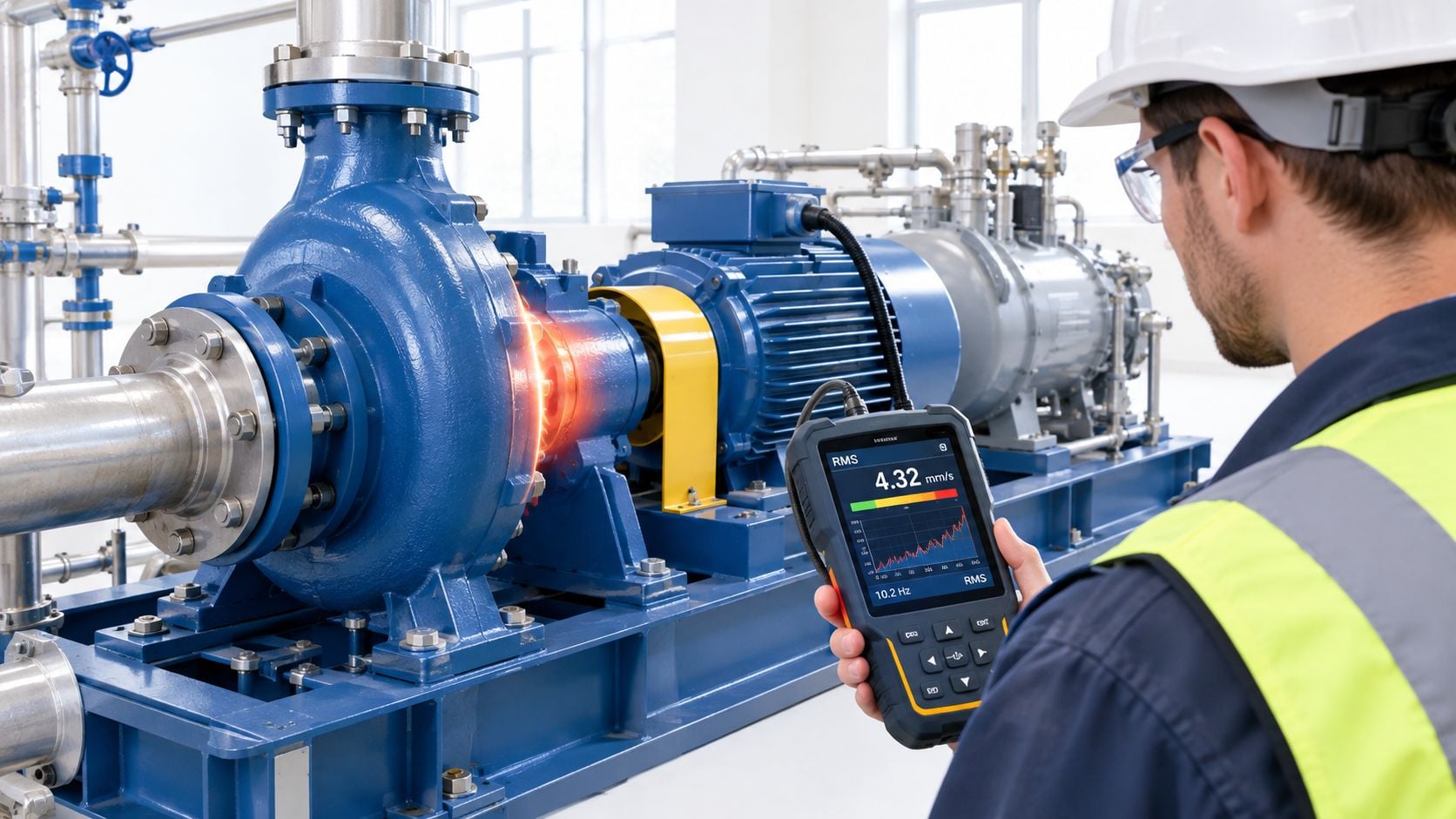
A process pump shows a progressive rise in vibration RMS, with the spectrum indicating a developing rolling-element bearing defect. The failure mode is not “pump failure” in general. It is bearing degradation that may progress into shaft damage, seal damage, or a forced shutdown.
The reliability engineer assigns a low band for the next short inspection window, a moderate band for the following window if the trend continues, and a high band for the longer operating horizon if no intervention occurs. The work orders follow the bands:
- Low band: continue operation, verify sensor repeatability, check lubrication and alignment, and shorten the route review.
- Moderate band: schedule a bearing inspection or replacement during the next feasible outage, with a contingency for accelerated degradation.
- High band: remove the pump from normal duty if the consequence justifies it, or transfer load to an available standby while completing the repair.
The thresholds aren't universal. They should be calibrated to vibration severity, trend slope, process criticality, and the time required to obtain parts and labor. A centrifugal pump reliability and failure prevention resource can help organize those failure modes around inspection and corrective actions.
Motor insulation degradation
A motor shows thermal asymmetry after repeated surge events, while thermography identifies a growing temperature difference between phases. The assumed failure mode is winding insulation breakdown, not merely “motor age.” A motor-current signature review, resistance testing, surge testing, load verification, and thermal follow-up can determine whether the signal reflects electrical stress, imbalance, loose connections, or an external load issue.
A stable temperature pattern with no corroborating electrical evidence supports continued operation and planned monitoring. A persistent delta combined with abnormal current and a history of surge exposure moves the motor into a higher action band, potentially requiring a rewind decision or a controlled replacement before the next production-critical run.
Screw compressor valve plate wear
A screw compressor with declining capacity, abnormal discharge temperature, and repeated valve-related findings presents a wear-out case. The estimate should cover the valve plate failure mode over a defined operating window and include the consequences of lost compressed-air capacity, secondary damage, and the availability of a backup compressor.
The practical choice may be to keep running under enhanced monitoring if the risk remains manageable, schedule refurbishment during a planned outage, or replace the worn assembly before secondary damage develops. Generic MTBF doesn't distinguish those choices. A named failure mode, condition evidence, time window, and consequence do.
How Probability of Failure Fits Into RBI and FMEA
Risk-Based Inspection, or RBI, combines probability of failure with consequence of failure. Consequence includes the effect on people, environment, production, equipment, and compliance. The combination creates a risk ranking that helps the plant decide where inspection resources should go.
Failure Modes and Effects Analysis, or FMEA, approaches the same decision from the failure-mode level. Probability of failure informs the occurrence rating. Severity represents consequence. Detection reflects the chance that existing controls will identify the problem before the effect occurs. A high occurrence rating with weak detection deserves a different task from a low occurrence event that is easily found during routine rounds.
The statistic becomes policy when it changes the task:
- Rising bearing risk may justify vibration analysis at a shorter interval.
- Insulation risk may justify thermography and electrical testing before a planned outage.
- Compressor wear may justify performance testing tied to a repair trigger.
- A low-consequence failure may remain run-to-failure if the plant can restore it quickly and safely.
The table below illustrates the structure without pretending that one interval fits every facility.
| Equipment | Time-Based Interval | PoF Estimate | Risk-Based Task | Detection Method |
|---|---|---|---|---|
| Centrifugal pump | Fixed bearing replacement schedule | Increasing risk for bearing defect over the next operating window | Trend vibration, verify lubrication, and schedule replacement when the action band is reached | Vibration analysis and oil inspection |
| Induction motor | Calendar-based electrical inspection | Conditional risk linked to thermal and electrical evidence | Escalate testing after abnormal temperature or surge exposure | Thermography, motor current, and electrical tests |
| Screw compressor | Fixed overhaul interval | Increasing risk for valve plate wear under degraded performance | Combine performance testing with planned refurbishment timing | Discharge temperature, capacity, and acoustic inspection |
An RBI program should also account for inspection effectiveness. A low probability estimate doesn't eliminate risk when detection is poor and consequence is severe. Conversely, a condition-monitoring task may reduce uncertainty enough to defer intrusive work, but only if the sensor, route, analyst, and response process can operate before the risk changes.
Teams building a broader risk vocabulary can consult these IT risk management resources, particularly when explaining likelihood, consequence, controls, and residual exposure to finance or operations. The industrial version still requires equipment-specific failure modes and evidence.
Limitations and Common Mistakes to Avoid
Probability models fail most often through false precision. A small sample can produce a clean-looking curve even when the plant has mixed designs, inconsistent duty, incomplete records, and multiple failure mechanisms. A surviving pump isn't proof of reliability, and a repaired pump may no longer belong to the same population after a major redesign or operating change.
Censoring creates another trap. Assets that have not failed by the end of observation carry information, but they aren't failed observations. Removing them can make the fitted population appear less reliable than the evidence supports. Combining seal failures, bearing failures, process trips, and operator-induced damage under one “pump failure” code produces a number that is easy to calculate and difficult to defend.
Operating conditions can overturn the nominal estimate
The 1986 Space Shuttle Challenger disaster remains a severe warning about the difference between design-assumed risk and evidence under actual conditions. NASA management reportedly treated catastrophic Shuttle failure probability as approximately 1 in 100,000, or 0.001%, while a contractor study estimated launch-loss risk between 1 in 1,000 and 1 in 10,000, or 0.1% to 0.01%. The solid-fuel rocket boosters were assigned a failure rate of about 1 in 40, or 2.5%, in the cited risk analysis (NASA's probabilistic risk analysis record).
Challenger broke apart 73 seconds after launch when an O-ring in the right solid rocket booster failed. A later probabilistic risk analysis estimated overall Shuttle failure probability at roughly 1 in 100, or 1%, while separate statistical analysis estimated O-ring seal failure probability at approximately 99.98% at 29°F, the relevant launch temperature range, using the evidence and assumptions described in the NASA record.
The lesson for a plant is direct. A probability based on nominal design expectations is not equivalent to probability under actual temperature, load, maintenance, contamination, or installation conditions.
Recall doesn't equal economic value
Predictive-maintenance research using an industrial CNC dataset distinguished random failures, defined in that example as a 0.1% probability independent of process variables, from deterministic failures associated with observable operating conditions. In the same test set, 66 of 2,000 machines experienced deterministic failures, a 3.3% rate; a model detected 54 of them, or 81.8% recall, while generating 346 false positives (the CNC predictive-maintenance study).
That result exposes the false-positive storm. A model can detect most relevant events and still overload planners, technicians, inspection routes, spare-parts decisions, and outage capacity. Thresholds should reflect the cost of a missed failure, the cost of an unnecessary intervention, and the time available to act. Accuracy and recall are model metrics. They aren't maintenance strategies.
A 2025 NIST review screened 465 peer-reviewed condition-monitoring studies published from 2001 through 2023 and found 42 eligible for detailed evaluation. The review reported comparatively few evaluation studies in manufacturing, incomplete descriptions of monitoring and maintenance models, and difficulty comparing results because economic metrics, performance measures, and uncertainty analyses varied (NIST's condition-monitoring evaluation review).
Probability of failure is credible only when its data, assumptions, calibration, and cost model are visible.
Validating Probability Estimates and Next Steps
A reliability team should backtest probability bands against actual failures, inspection findings, and post-maintenance outcomes. It should demand confidence intervals rather than point estimates, calibrate alerts using cost-sensitive thresholds, and review whether each alert created the right work order at the right time. Strong recall numbers aren't enough if the model increases false work, misses the intervention window, or fails to reduce unplanned downtime.
A practical next step is a no-cost assessment of one critical pump, motor, or compressor, with the failure mode, condition evidence, inspection interval, and consequence model documented before any probability number is accepted.
Forge Reliability applies vibration analysis, oil analysis, thermography, ultrasound, motor-current analysis, Weibull methods, FMEA, and criticality ranking to specific plant assets. Visit Forge Reliability to request a free reliability assessment and a 24-hour response from plant-floor specialists who can turn probability estimates into defensible inspection intervals and work orders.