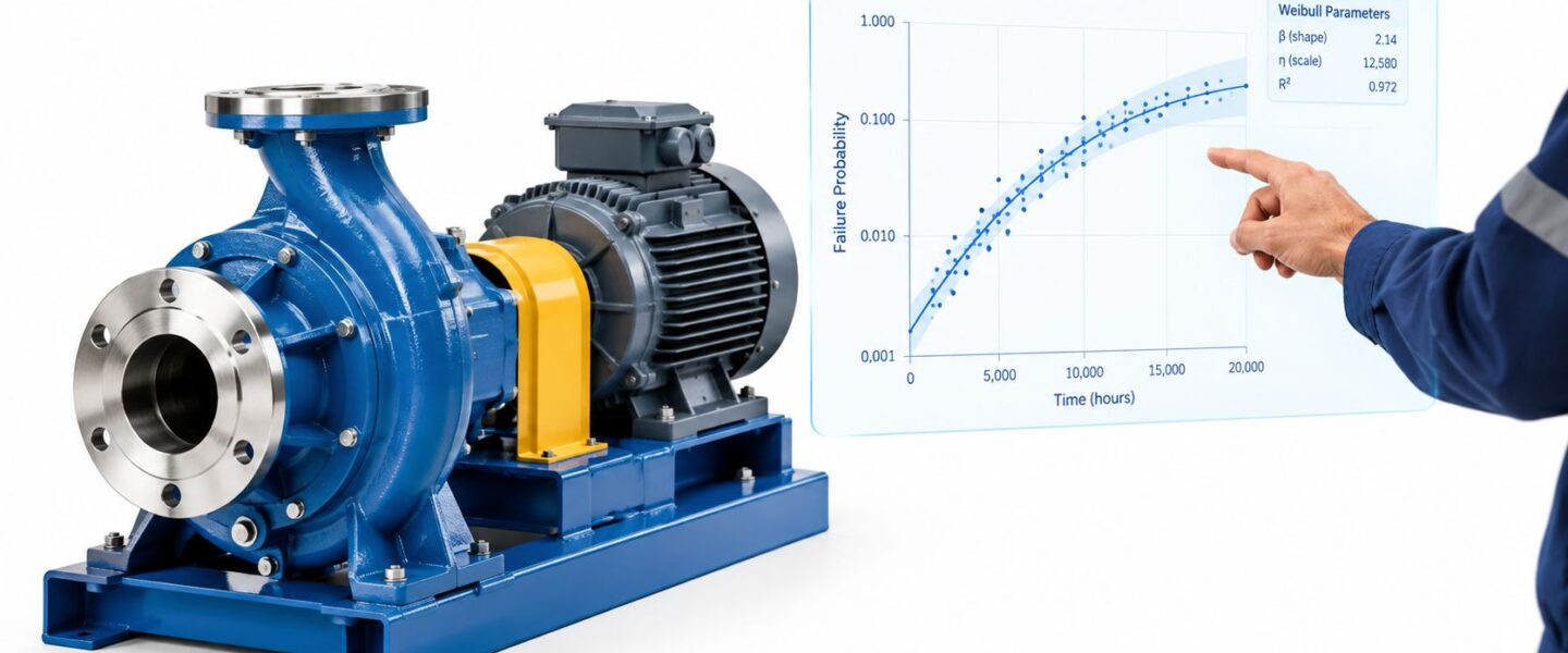
A centrifugal pump on a chemical processing line fails again, but the maintenance record says only “bearing failure.” One unit has run continuously, another has spent weeks in standby, and a third was removed during an inspection while it was still operating. If those events are sorted by calendar date and the survivors are omitted, the resulting Weibull curve can look neat while describing the wrong population.
That is the practical problem behind Weibull analysis reliability. The model can help determine whether a failure pattern points to infant mortality, random failure, or wear-out, but it can't rescue poor failure-mode coding, mixed duty cycles, or incomplete exposure data. A defensible result depends less on producing a curve than on knowing whether the curve deserves a maintenance decision.
Table of Contents
- Why Weibull Analysis Matters for Industrial Reliability
- Preparing Life Data That Will Not Mislead Your Model
- Fitting the Weibull Model and Reading the Probability Plot
- Interpreting Beta and Eta for Maintenance Strategy
- Worked Example Turning Pump Data Into PM and Spares Decisions
- Avoiding Costly Pitfalls and Getting Your Next Assessment
Why Weibull Analysis Matters for Industrial Reliability
A pump bearing fails after a short run. The immediate response might be tighter installation control, alignment checks, lubrication review, or contamination prevention. If the same bearing population fails progressively with age, condition monitoring or planned replacement may be justified. A random-looking pattern points elsewhere, often toward process upsets, protection gaps, or external causes that an age-based replacement will not address.
Weibull analysis reliability gives the reliability team a common framework for separating these patterns. It uses the shape parameter β and scale parameter η to describe decreasing, roughly constant, or increasing failure-rate behavior. That connection can support decisions about quality improvement, inspection, condition monitoring, and replacement planning. In practice, the parameters classify observed behavior. They do not identify the root cause or authorize a maintenance interval by themselves.

Operating exposure matters more than the date on the work order
Calendar time becomes misleading when duty varies. A standby pump, a batch-operated pump, and a continuously loaded pump may have the same installation date but very different mechanical exposure. Operating hours, starts, load cycles, or another physically relevant exposure measure usually gives the failure time more meaning than elapsed calendar time.
Keep units that have not failed in the dataset. These right-censored observations show that an asset survived to a recorded exposure, although its eventual failure time remains unknown. Removing them makes the failed units appear more representative and can shift the estimated failure pattern.
Sparse field data needs restraint. A probability plot may look convincing even when only a few failures are observed and many units are censored. Treat the fitted curve as directional when confidence limits are wide, failure-mode coding is uncertain, or exposure histories are inconsistent. Do not change a PM interval on fit quality alone. Check consequence, failure-mode evidence, uncertainty, and the practical gap between the proposed interval and the observed lives.
Split the population when mechanisms or duty cycles differ materially. One curve can conceal early installation defects in one group and age-related wear in another. A separate analysis, or a decision to collect more data, may be more defensible than forcing unlike observations into one model.
For broader reliability work, RBI FMEA RCA and RCM for drive connects Weibull decisions with risk-based inspection, failure-mode analysis, root cause analysis, and reliability-centered maintenance. Review equipment failure patterns and the six curves before selecting a distribution or interpreting β.
Practical rule: Use a Weibull result when it improves a defined decision. With sparse censored data, a good fit can still support direction only. The correct output may be uncertainty, further inspection, or better failure-mode separation rather than a new maintenance interval.
Preparing Life Data That Will Not Mislead Your Model
The quality of a Weibull estimate is established before the software calculates β or η. Field records often contain suspected failures, corrective work, inspections, replacements, and repeated repairs. Those events don't automatically constitute life data.
Start by defining the population and the failure mode. “Pump failure” is too broad for a useful life model if it combines seal leakage, bearing damage, impeller erosion, motor winding faults, and process-induced trips. Each mechanism can have a different age relationship and a different corrective action.
Build the dataset as a controlled audit
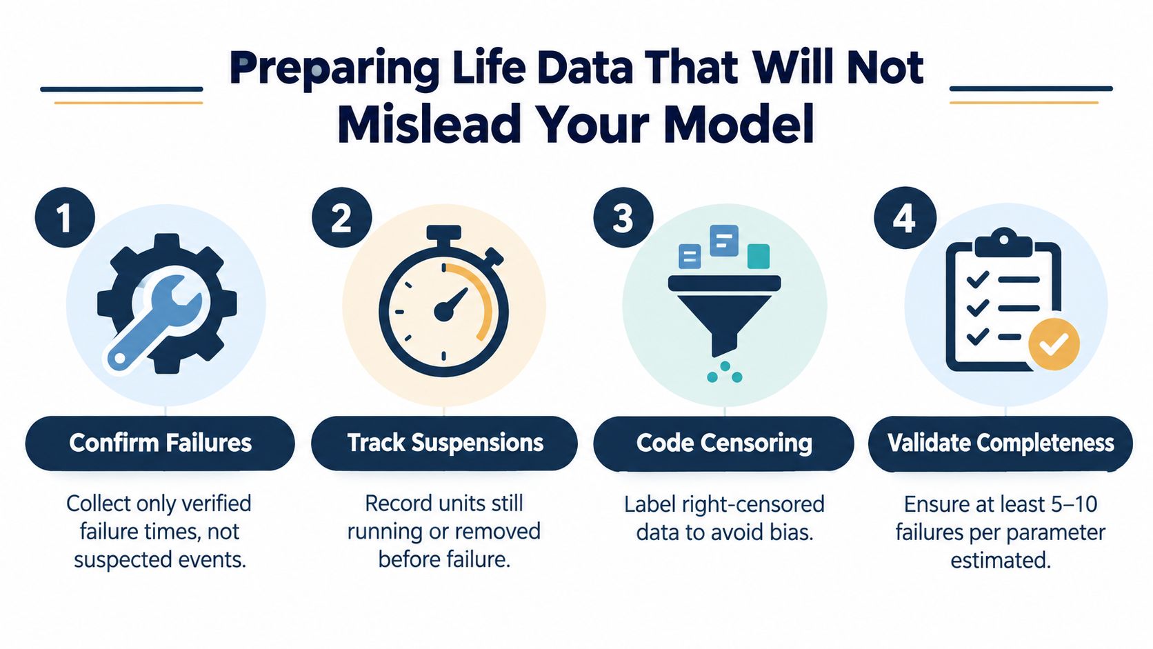
A practical preparation workflow is:
- Confirm failures. Include only events supported by inspection, teardown, diagnostic evidence, or a reliable failure code. A work order that says “bearing replaced” doesn't prove the bearing was the initiating failure.
- Track suspensions. Record assets still operating at the end of observation and assets removed for reasons other than the target failure. These are censored observations, not missing failures.
- Measure exposure consistently. Use operating time where it reflects the mechanism. For a pump bearing, that may be run hours; for equipment dominated by starts and stops, cycles may be more appropriate.
- Rank the observations correctly. Sort confirmed failures and suspensions by exposure time, then preserve each observation's event status.
- Check the population boundary. Don't combine assets with materially different designs, lubrication arrangements, duty cycles, installation practices, or process conditions unless the failure mechanism is demonstrably common.
A maintenance team should also separate life data from repairable-system event data. If a bearing is replaced and the same pump returns to service, the next bearing's life isn't automatically a continuation of the first component's life. Treating every corrective work order as an independent component life can create a dataset that describes repair frequency rather than time to first failure.
Use the CMMS export as evidence, not truth
Before fitting, reliability engineers should review:
- Asset identity: Is each record tied to the correct pump, motor, bearing position, and configuration?
- Failure confirmation: Does the failure code identify the failed component and mechanism?
- Exposure basis: Are hours, cycles, or another measure available and applied consistently?
- Censoring status: Can the analyst distinguish failed units from survivors and removals?
- Duplicate events: Have follow-up repairs, inspection findings, and repeat work orders been separated?
- Population consistency: Are site, duty, process, and design differences documented?
Mean time between failure is a different measure from component life, especially for repairable systems. Teams reviewing that distinction can use this explanation of how to calculate mean time between failure before deciding whether a CMMS export is suitable for Weibull analysis.
The failure-mode coding step is where many industrial datasets fail. A broad label hides mechanism changes, while an over-specific code can leave too few observations to estimate anything useful. The right level is the one that supports a distinct engineering action, such as lubrication control for bearing distress or contamination control for seal damage.
Fitting the Weibull Model and Reading the Probability Plot
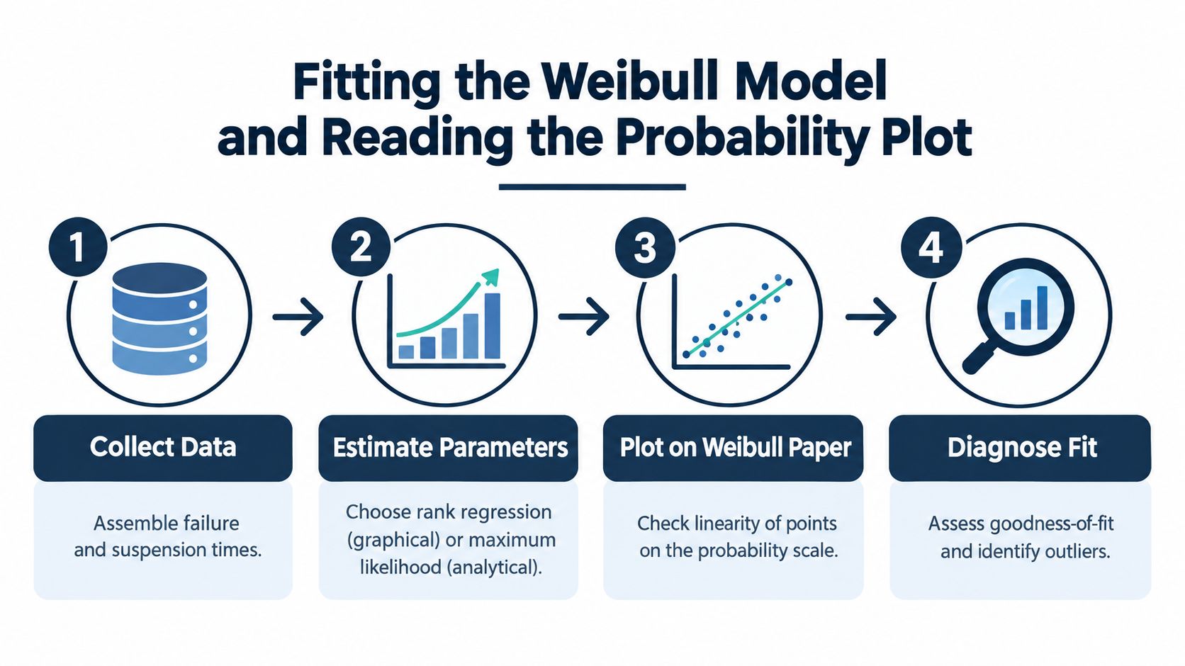
Once the life data has been audited, choose an estimation method that matches the evidence. Rank regression fits a line to transformed plotting positions and can support exploratory work with complete data. Maximum likelihood estimation, usually called MLE, estimates parameters by finding the values that make the observed failures and suspensions most plausible. MLE handles censoring more directly, but it still depends on correct model setup, exposure definitions, and suitable Weibull analysis software.
A fitting method cannot correct a mixed population. Combining seal leaks, bearing defects, and impeller erosion may produce a neat mathematical line with little maintenance value. The probability plot is a diagnostic surface. Use it to test whether the records belong in one population before using its slope or characteristic life to change a PM interval.
Read the pattern before accepting the parameters
A roughly straight pattern on Weibull probability paper supports the selected distribution for the analyzed population. Curvature, clusters, or a visible knee require investigation. They can indicate mixed failure modes, changing operating conditions, separate asset groups, or a shift between early and later failure behavior.
A good fit is still only directional when the field sample is sparse and heavily censored. A line may look convincing because many units have not failed, while the actual failure mechanism remains uncertain. Do not treat that plot alone as proof that a new PM interval will reduce risk.
If the points do not follow an approximate line, review the failure codes and operating context. Split the records by failure mode when the mechanisms lead to different actions. Split by duty cycle when load, temperature, speed, or process service changes the expected life. Keep one curve only when the groups share a defensible population and the combined result supports the decision.
Treat confidence bounds as part of the result
A point estimate of β or η hides sampling uncertainty. Confidence bounds show how widely the parameters could vary given the available evidence, and that range belongs in every PM, replacement, or spares decision. With few failures and many suspensions, the bounds can remain wide even when the plotted points appear orderly.
Basic Weibull estimation generally needs roughly 15 to 20 failures for an initial evidence base. Decision-grade maintenance planning often calls for roughly 30 to 50 failures, while tighter comparisons and detection of small improvements may require 100 or more failures. Results based on fewer than 5 failures are commonly treated as exploratory rather than actionable. These thresholds do not replace review of failure mechanism, censoring pattern, confidence bounds, or asset criticality.
The fit can be good while the decision is weak. A straight line with broad confidence bounds remains a directional result.
Before acting, ask three questions. Does the selected population have a coherent failure mechanism? Does the fitted line describe the observed range without obvious curvature? Are the parameter bounds narrow enough for the consequence of the proposed maintenance change? If the final answer is no, use the model to guide data collection and investigation, not to justify a confident PM change.
Interpreting Beta and Eta for Maintenance Strategy
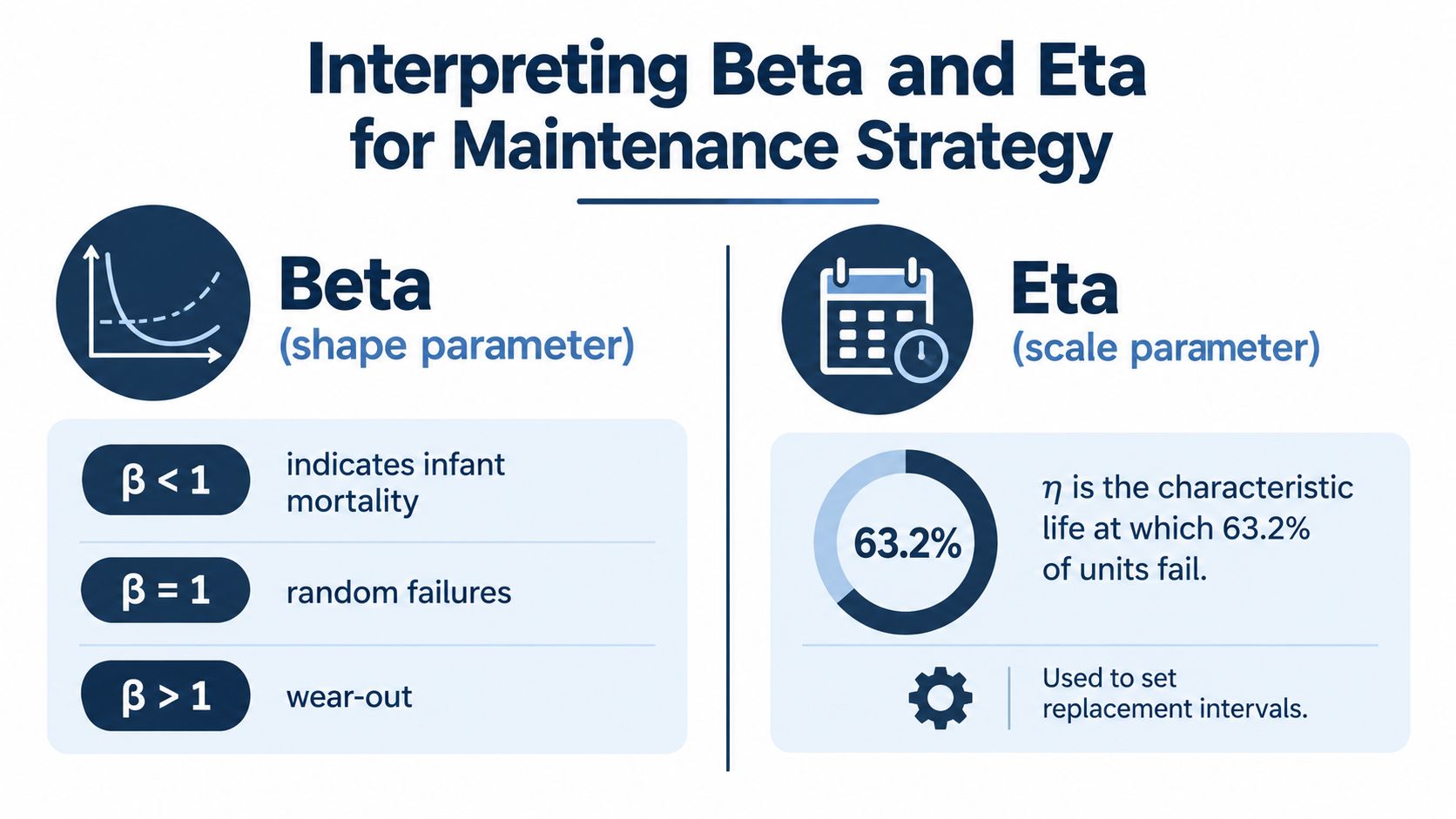
A Weibull fit can look orderly while the maintenance decision remains uncertain. The shape parameter β describes the modeled failure-rate pattern, not the physical cause by itself. A value below one is consistent with decreasing failure rate and infant-mortality behavior. A value near one is consistent with random failure. A value above one is consistent with increasing failure rate and wear-out.
The scale parameter η, or characteristic life, marks the point at which approximately 63.2% of the modeled population has failed. Use it to compare consistently defined asset groups or failure modes, such as pump bearings operating under different duty cycles. The comparison is defensible only when the groups share a credible failure mechanism. With sparse field records, censored observations, or mixed operating conditions, η should guide investigation rather than set a replacement date.
Beta and Eta Decision Matrix for Maintenance Actions
| Beta Range | Failure Pattern | Recommended Action | Example |
|---|---|---|---|
| β < 1 | Infant mortality | Investigate installation, manufacturing quality, alignment, lubrication, and commissioning controls. Avoid default age replacement. | A new pump bearing shows early damage after poor lubrication or incorrect fit. |
| β = 1 | Random failures | Prioritize condition monitoring, protection, process controls, and root cause analysis. Age-based replacement may add little value. | A bearing fails after unrelated process upsets with no consistent age pattern. |
| β > 1 | Wear-out | Evaluate condition monitoring, planned replacement, inspection timing, and spare-parts coverage. Confirm that the wear mechanism is physically credible. | Rolling-element bearing damage increases with operating age. |
Translate parameters into actions carefully
A high β may support an age-related strategy when the population is stable, the failure mode is confirmed, and confidence bounds are narrow enough for the consequence of the change. It still does not make η a guaranteed safe life. Set an intervention interval using consequence, inspection or detection capability, uncertainty, and the cost of planned work.
A β below one directs attention to early defects. Review shaft alignment, controlled fits, lubricant cleanliness, storage, commissioning, and supplier quality. A β near one generally shifts effort toward vibration monitoring, lubrication analysis, operating protection, and failure investigation instead of calendar replacement.
Do not fit one curve across materially different failure modes or duty cycles. Splitting the data may produce fewer observations, but a smaller coherent group is often more useful than a larger mixed population. If the split leaves only a handful of failures, treat β and η as directional and collect better evidence before changing PM intervals.
For an individual asset, remaining useful life analysis can complement the population model. Weibull parameters describe group behavior, while condition data helps assess the asset's current state.
Worked Example Turning Pump Data Into PM and Spares Decisions
A chemical processing line has several centrifugal pumps with recurring motor-side bearing replacements. The maintenance manager wants a shorter planned replacement interval, but the records include operating pumps, removed pumps, and failures coded only as “bearing issue.” The reliability engineer first narrows the analysis to one bearing position and one confirmed failure mode, bearing damage verified by inspection.
Step one defines the evidence
The team exports each unit's operating exposure, failure status, failure mode, and configuration. Operating hours are used instead of calendar age because the pumps run under different production schedules. Units still operating at the end of the review period remain in the dataset as suspensions, and units removed for inspection or configuration change are also classified according to why observation ended.
The analyst ranks the exposure times from shortest to longest and checks every event against the work order, inspection note, and teardown evidence. Repairs to other components are excluded from this component-life dataset. A record saying “pump overhauled” isn't treated as a bearing failure unless the bearing damage is confirmed.
The dataset is then divided by duty cycle if process conditions differ materially. A pump serving a steady process stream shouldn't automatically be pooled with one exposed to intermittent starts, contamination, or a different load profile. Pooling is acceptable only when the failure mechanism is common and the operating exposure is comparable.
Step two fits the censored data
Because the dataset contains suspensions, the engineer uses maximum likelihood estimation rather than relying only on a graphical fit. The output includes β, η, confidence bounds, the observation range, and a probability plot. The plot is checked for curvature and a knee, not just for whether the fitted line appears visually acceptable.
Suppose the estimated β is above one, suggesting a wear-out pattern, but the confidence bounds are broad because the confirmed failure count is small. That combination supports a cautious interpretation: bearing wear may be increasing with exposure, but the evidence isn't strong enough to impose an aggressive replacement interval across every pump.
The engineer also checks whether η lies within or near the observed exposure range. Extrapolating far beyond observed lives makes a maintenance interval look more precise than the data can support. If the proposed interval sits well beyond the evidence, it should remain a planning hypothesis until more failures, suspensions, or controlled test data improve the basis.
Step three chooses a controlled maintenance response
The plant doesn't immediately replace all bearings at η. Instead, it introduces a staged response:
- Inspection first: Increase attention to vibration, bearing temperature, lubrication condition, alignment, and contamination indicators on the critical pumps.
- Targeted replacement: Use planned replacement only where the wear-out interpretation is physically credible and the consequence of failure justifies intervention.
- Data improvement: Require failure confirmation, operating-hour capture, and consistent bearing failure codes on every future event.
- Review trigger: Recalculate the model when additional evidence changes the observed failure pattern or materially narrows the uncertainty.
The PM interval is documented as provisional, with the fitted parameters, confidence bounds, censoring treatment, exclusions, and rationale attached to the maintenance plan. That record prevents a directional estimate from becoming an undocumented standard.
Step four links the model to spares
Spares planning shouldn't use η as a direct stocking quantity. The planner combines the directional failure pattern with pump criticality, supplier lead time, interchangeability, existing inventory, repair capacity, and the consequence of an unavailable bearing. A wear-out indication may justify greater readiness for the affected bearing, but the quantity decision remains an operational risk decision rather than a simple Weibull output.
The same analysis can inform an RCM task. If bearing distress is detectable before functional failure, vibration or lubrication monitoring may be more defensible than routine replacement. If detection is weak and the consequence is severe, a planned intervention may still be considered, but the uncertainty must be made explicit.
For additional pump-specific prevention ideas, the team can consult this resource on centrifugal pump reliability and failure prevention. The central discipline remains unchanged: use the model to narrow choices, document assumptions, and avoid presenting a sparse field estimate as a guaranteed life limit.
Avoiding Costly Pitfalls and Getting Your Next Assessment
The most dangerous Weibull mistake isn't a calculation error. It's treating a good fit as proof that the maintenance decision is valid. A model can fit a mixed or poorly defined dataset while concealing the fact that calendar time replaced operating exposure, survivors were excluded, or repairable-system events were mistaken for component lives.
Several failure modes repeatedly create false precision:
- Sparse evidence: Small samples can make β and η unstable, so point estimates shouldn't drive major PM changes without confidence bounds.
- Mixed mechanisms: A single curve can hide seal leakage, bearing wear, contamination, and process upset failures that require different actions.
- Duty-cycle blending: Combining standby and continuously operating pumps can create a population with no coherent exposure basis.
- Overextended forecasts: Maintenance intervals projected far beyond the observed range can appear exact without being well supported.
- Unverified fit: A straight probability plot doesn't prove that the chosen failure mode, population, or decision threshold is appropriate.
Know when standard Weibull is too simple
Modern industrial assets often experience multistage failures, changing process conditions, and higher-order system behavior. A study of industrial pumping systems published in 2026 proposes a Weibull reliability approach using six higher-order methods, a signal that complex pumping applications may require more than one conventional distribution. The study is relevant not because every plant should adopt an advanced method immediately, but because it challenges the assumption that one curve always represents one asset population.
The practical response is segmentation before sophistication. Separate by failure mechanism, duty cycle, site, design, or operating regime when engineering evidence supports those distinctions. If the groups become too small, keep the model directional and improve the data rather than manufacturing certainty.
Decision discipline: If the uncertainty is wider than the maintenance consequence can tolerate, don't convert the estimate into a permanent PM interval.
A free reliability assessment can review whether field data is strong enough to support an interval change, whether suspensions and failure modes are coded correctly, and whether a pump population needs segmentation. Forge Reliability also applies Weibull analysis alongside condition monitoring, FMEA, RCM, criticality ranking, and CMMS data governance, so the statistical result can be tested against the physical failure mechanism.
Forge Reliability can review a plant's pump and rotating-equipment life data, identify censoring and failure-mode weaknesses, and determine whether Weibull outputs should guide PM changes or remain advisory. Visit Forge Reliability to request a free reliability assessment focused on defensible maintenance intervals, condition-monitoring tasks, and spares decisions.