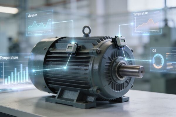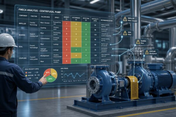
A maintenance manager reviews a vibration trend and sees a clean, stable line. The baseline looks convincing, so alarm limits are approved and the route is released. Weeks later, the same centrifugal pump alarms at a different flow condition, even though the machine may be operating normally. The problem began before the first threshold was calculated. The reference data described a convenient moment, not the machine's real operating envelope.
Baseline data collection is the technical foundation for anomaly detection, condition monitoring, and predictive maintenance. If technicians capture unstable startup readings, measurements from a machine with an existing fault, or too few samples to represent normal variation, every downstream decision inherits that error. A defensible baseline requires a known-good asset, repeatable measurement methods, documented operating context, and a reference that can be compared meaningfully with future readings.
Table of Contents
- Why Most Baselines Fail Before Monitoring Even Starts
- Planning a Baseline Project That Will Hold Up
- Matching Instruments to the Failure Modes You Care About
- Building a Sampling Plan With Real Numbers
- Turning Baseline Statistics Into Working Thresholds
- Wiring Baselines Into CMMS and Continuous Monitoring
- Common Baseline Mistakes and How to Recover
Why Most Baselines Fail Before Monitoring Even Starts
A centrifugal pump in a process plant provides a familiar example. The maintenance team captured its initial vibration data on a hot afternoon, while strainers were partially clogged and flow through the branch was low. The coupling also had slight misalignment from the previous teardown. The route readings looked tidy because the machine was measured under one narrow condition, not because the asset was healthy across its duty range.
The team used those readings to set thresholds. Six weeks later, the pump generated an alarm at another operating point that had never been sampled. Operators treated the event as a monitoring problem, but the failure was in the baseline design. The original reference had understated normal variability and had included mechanical and process conditions that should have been corrected or excluded.
Three patterns create most of this damage:
- Unrepresentative operating states: A reading taken at low flow, unusual load, abnormal temperature, or altered process conditions may not describe normal operation.
- Transient contamination: Startup, warm-up, shutdown, and coastdown data can contain temporary vibration and temperature behavior that shouldn't define steady-state limits.
- Thin sampling: A few readings from one duty cycle can make the machine appear more stable than it is.
Why the error propagates
A baseline becomes the reference for future anomaly detection. Canadian engineering guidance explains that, without a starting point, monitoring data can't reliably support residual-life prediction, and it identifies repeatability as the central requirement for useful baseline data. The same guidance recommends designing condition databases so tests remain repeatable despite operator, weather, and ambient variation, which makes baseline quality a technical control rather than a paperwork exercise. (Canadian engineering guidance on predictive-maintenance baselines)
A bad reference affects more than a dashboard. It shifts advisory limits, changes severity classification, trains anomaly-detection models on contaminated behavior, and can produce either nuisance alarms or missed bearing wear. A pump with early looseness may be labeled healthy if the baseline captures the defect, while a normal high-load condition may be labeled abnormal if the reference never included it.
Practical rule: A baseline is valid only when the asset is known to be healthy, the operating state is representative, and another technician can repeat the measurement.
Teams building a condition monitoring system should treat the baseline as a living reference. Process changes, overhauls, sensor replacement, and changes in duty cycle can all require a review or a new qualified reference.
Planning a Baseline Project That Will Hold Up
The planning sequence matters more than the first route sheet. Before collecting a single reading, the reliability team should decide which assets deserve attention, what failure modes matter, where sensors will be placed, and what makes a sample acceptable.
Start with criticality multiplied by redundancy. A high-consequence pump with no standby should be baselined before a less critical motor that has an available spare. Criticality should reflect safety, environmental exposure, production impact, repair difficulty, and the consequences of a hidden failure. Redundancy changes the decision because a standby asset may reduce immediate production risk, while a single process pump can become a bottleneck.
The running example is a pump and motor pair. The team should identify the pump bearings, motor drive-end and non-drive-end bearings, coupling, base, and connected piping as separate measurement points. ISO 17359 defines baseline data as measurements taken when equipment operation is acceptable and stable, and notes that machines with multiple operating states may need separate baselines. (ISO 17359 condition-monitoring guidance)
Decide the measurement system
Instrument selection should follow the failure modes and the applicable machine-monitoring framework, including ISO 10816, ISO 17359, and, where relevant, API 670 protection requirements. A pump and motor route may use an ICP accelerometer for vibration, a velocity sensor for overall machine severity, and a current clamp for electrical screening. The transducer's frequency range must cover the diagnostic objective, not merely the instrument's marketing specification.
Sensor locations need to be fixed before the route begins:
- Pump drive-end bearing, radial and axial directions.
- Pump non-drive-end bearing, radial and axial directions.
- Motor drive-end bearing, radial and axial directions.
- Motor non-drive-end bearing, radial and axial directions.
- Coupling-side locations where misalignment and looseness can transfer energy.
The team should also define acceptance criteria for runout, signal-to-noise ratio, repeatability, operating-point coverage, environmental notes, lubricant temperature, and steady-state confirmation. A one-page checklist per asset should name the responsible technician, analyst, operations contact, and approver.
| Decision | Pump Example | Motor Example | Acceptance Criteria |
|---|---|---|---|
| Criticality | Single process pump with limited redundancy | Motor driving the pump | Ranking approved before collection |
| Instrument | ICP accelerometer and velocity measurement | Accelerometer, velocity measurement, current clamp | Calibration status verified |
| Sensor locations | Drive-end, non-drive-end, radial, axial, coupling side | Drive-end and non-drive-end, radial and axial | Locations marked and repeatable |
| Operating states | Normal flow and documented load conditions | Matching load and speed conditions | State confirmed by operations |
| Sign-off | Reliability engineer and pump owner | Electrical and mechanical representatives | Method, data, and exceptions approved |
A clean plan prevents a common mistake: collecting technically precise measurements that answer the wrong question.
Matching Instruments to the Failure Modes You Care About
No condition-monitoring technique sees every failure mode. The correct baseline combines methods only where each method adds diagnostic value.
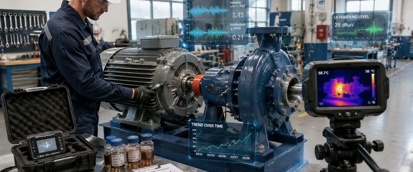
Vibration is the primary tool for imbalance, misalignment, mechanical looseness, and rolling-element bearing defects. It can cover a broad diagnostic range from 10 Hz to 10 kHz, but it remains sensitive to sensor mounting, speed, load, structural transmission, and the selected frequency band. A radial accelerometer near a pump bearing can identify changes that a motor terminal reading won't show. Practical guidance on how to measure vibrations helps standardize direction, location, and collection technique.
Infrared thermography identifies electrical hotspots, steam-trap problems, and cooling loss caused by low flow. It is useful at motor terminals, electrical connections, bearing housings, heat exchangers, and steam-system components. It won't reliably expose a mechanical defect hidden inside a sealed gearbox if surface temperature hasn't changed enough to distinguish the fault.
Oil and wear-debris analysis can identify gear-tooth scuffing and bearing fatigue particles before vibration rises. The sample location matters. A drain sample may not represent the active lubrication zone, and an unflushed sample valve can introduce contamination. Oil temperature, lubricant grade, filter changes, and recent maintenance must travel with the result.
Airborne and structure-borne ultrasound helps detect slow-speed bearing defects, steam leaks, and partial discharge. It is valuable where vibration energy is weak or where leak detection has a direct operational benefit. It can be affected by access, background noise, surface condition, and operator technique.
Motor current signature analysis, or MCSA, examines electrical current behavior in induction motors running at line frequency. It can screen for rotor-bar problems and air-gap eccentricity, but it shouldn't replace mechanical vibration data for coupling, bearing, or pump hydraulic faults.
| Technique | Primary Failure Modes | Blind Spots | Sensor Placement |
|---|---|---|---|
| Vibration | Imbalance, misalignment, looseness, bearing defects | Process causes without mechanical response, poor access | Bearing housings, coupling side, radial and axial directions |
| Thermography | Electrical hotspots, steam-trap failure, low-flow cooling loss | Internal mechanical defects in sealed enclosures | Terminals, housings, traps, electrical panels |
| Oil analysis | Gear scuffing, bearing fatigue particles, contamination | Dry assets, poor sampling points, non-lubricated faults | Active lubrication circuit, drain or dedicated sample port |
| Ultrasound | Slow-speed bearing defects, steam leaks, partial discharge | Limited access, strong background interference | Bearing housing, valves, steam components, electrical enclosures |
| MCSA | Rotor-bar faults, air-gap eccentricity | Most mechanical faults outside motor electrical behavior | Motor supply conductors or current measurement point |
Process variables complete the picture. For a pump, differential pressure combined with flow can distinguish a hydraulic operating change from a mechanical defect. A practical explanation of flow measurement with differential pressure is useful when pressure and flow need to be tied to the vibration record.
The best matrix isn't the one with the most sensors. It is the one that assigns each failure mode a detection method, a measurement point, and a known blind spot.
Building a Sampling Plan With Real Numbers
A defensible vibration baseline starts with a sampling rule that separates stable machine behavior from transient or poorly captured data. For the pump and motor pair, collect three repeat measurements per measurement point at three steady-state load conditions, such as 50%, 75%, and 100% of rated flow. Each vibration point needs a 10-second time-domain capture and at least 1,600 lines of frequency resolution for spectra below 2,000 Hz, following baseline sampling guidance for condition monitoring.
Phase-stable measurements should contain at least 20 revolutions for synchronous components. For non-synchronous peaks, use 10 averages so random noise does not dominate the result. These settings cannot correct an unhealthy machine, but they reduce the risk that acquisition settings conceal meaningful variation. Thin samples create another problem: a threshold or machine-learning model may treat one convenient reading as normal even though it came from an unusual load, startup transient, or unstable process condition.
List ISO 10816-3 and ISO 17359 in the project method statement. ISO 13373-1 defines baseline vibration around the machine's initial stable condition, preferably in normal mode and at normal flow rate. Measure the process pump after startup stabilization, not during transient warm-up, as described in ISO 13373-1 vibration guidance.
Gate every sample
Thermal imaging needs a separate acceptance rule. Keep the load within ±5% of the operating point and collect three frames per point. Reject images taken within 90 seconds of a process step change. Record lubricant temperature, ambient conditions, focus, emissivity, and process state with each accepted sample.
| Technique | Repeats per Point | Operating States | Capture Window | Acceptance Gate |
|---|---|---|---|---|
| Vibration | 3 | 50%, 75%, 100% rated flow | 10-second time record | Steady state, lubricant temperature, environmental notes |
| Vibration spectrum | 3 | Matching pump and motor states | 1,600 lines below 2,000 Hz | Signal-to-noise and repeatability accepted |
| Phase data | 3 | Stable speed and load | At least 20 revolutions | Phase stable |
| Non-synchronous analysis | 3 | Stable operating state | 10 averages | Peak remains distinguishable from noise |
| Thermography | 3 frames | Load within ±5% | Reject within 90 seconds of process step | Load, focus, emissivity, and process state recorded |
Keep failure and downtime definitions consistent in the route history. Anyone reviewing mean time between failure calculations should apply the same asset boundaries and event rules used in the baseline record. Otherwise, later reliability comparisons mix measurement quality with inconsistent maintenance reporting.
Turning Baseline Statistics Into Working Thresholds
Raw readings become useful only after qualified samples are grouped by measurement point, operating state, and frequency band. For each group, calculate the baseline mean, written as µ, and standard deviation, written as σ. The threshold scheme in this example uses advisory at µ + 2σ, alert at µ + 3σ, and alarm at µ + 4σ or the ISO 10816-3 zone boundary, whichever is lower. (Condition-monitoring threshold guidance)
Consider a 75 kW motor with a bearing-housing velocity baseline of 1.8 mm/s RMS and a standard deviation of 0.25 mm/s. The calculated limits are:
| Statistic | Formula | Value (mm/s) | Action |
|---|---|---|---|
| Baseline mean | µ | 1.8 | Reference condition |
| Standard deviation | σ | 0.25 | Normal variation |
| Advisory | µ + 2σ | 2.3 | Review trend and operating state |
| Alert | µ + 3σ | 2.55 | Schedule diagnostic investigation |
| Calculated alarm | µ + 4σ | 2.8 | Escalate for immediate assessment |
| ISO zone D ceiling | Boundary comparison | 4.5 | Use lower applicable limit |
The calculated alarm is 2.8 mm/s, which is lower than the 4.5 mm/s ISO zone D ceiling. That lower value governs this example because the asset-specific distribution indicates a meaningful change before the broader zone boundary is reached.
Use bands, not just broadband values
A broadband RMS threshold can remain stable while an early bearing defect grows inside a narrow frequency band. The 1× RPM band, meaning the frequency associated with rotational speed, should have its own baseline, such as 1× RPM ±2 Hz, because imbalance and misalignment energy may change independently from bearing tones.
Crest factor, the ratio of a signal's peak value to its RMS value, can expose impulsive events associated with early spalling before overall velocity moves noticeably. It should be trended alongside time waveform, spectrum, phase, temperature, and process load.
Thresholds belong to the asset record, not to a generic equipment class. After a major repair, redesign, coupling change, bearing replacement, or sensor replacement, the reliability team should document whether the existing reference remains valid. Distribution changes and threshold reviews can also support Weibull analysis software workflows when failure history is mature enough for life modeling.
Wiring Baselines Into CMMS and Continuous Monitoring
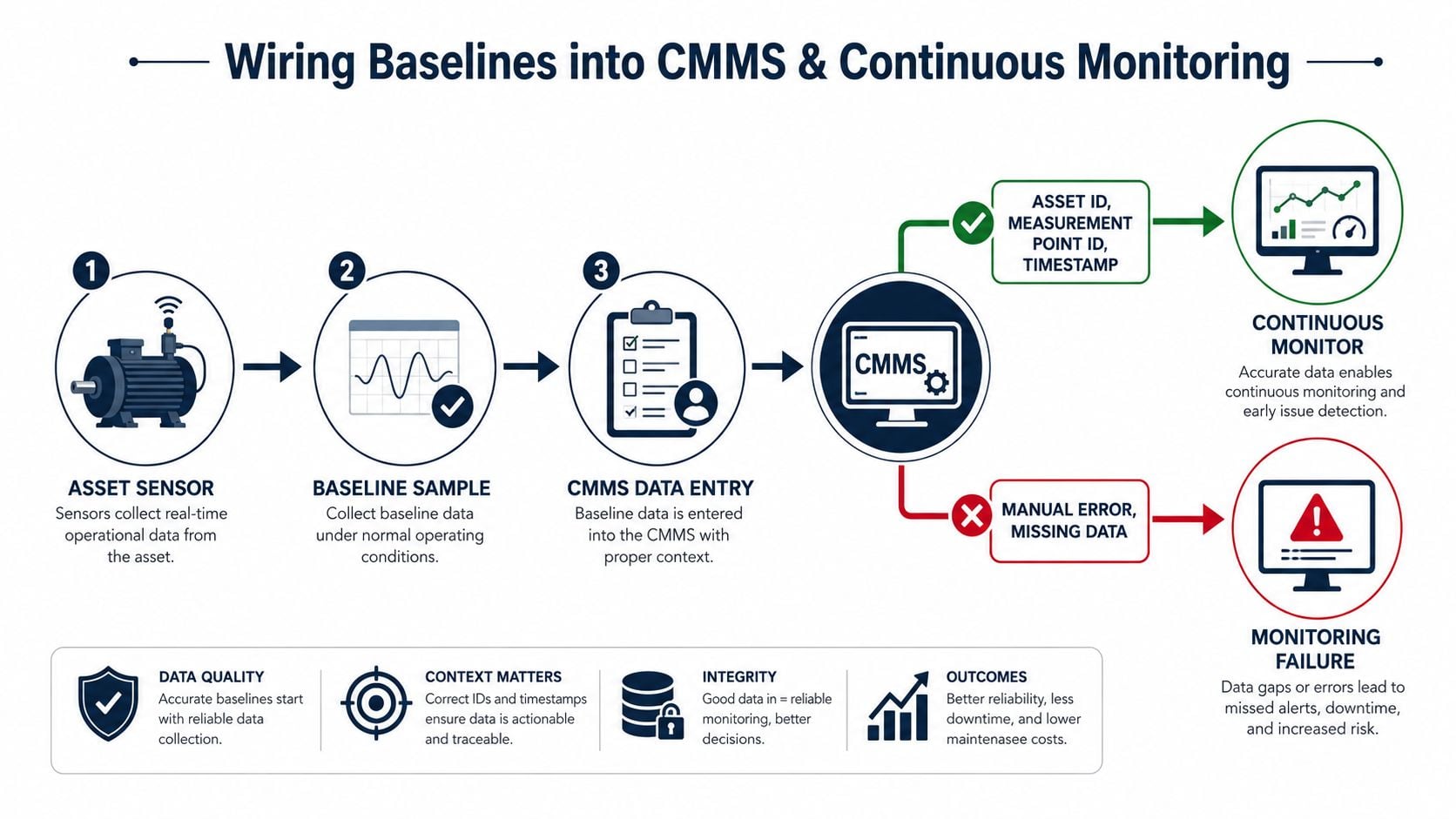
A gearbox and an air compressor show why data structure matters. A technician may collect an excellent gearbox bearing spectrum, but if the file is saved without the asset ID or operating state, the result becomes difficult to connect to a work order. An online compressor sensor can stream clean data, yet still produce misleading alerts if the system refreshes the baseline from every point, including startup and unloading transitions.
Each accepted sample should enter the CMMS with the same fields:
- Asset ID: The permanent equipment identifier.
- Measurement point ID: The exact bearing, terminal, valve, or sample port.
- Operating state: Load, speed, pressure, flow, and process mode where relevant.
- Instrument serial and calibration date: Proof that the measurement chain was controlled.
- Analyst and timestamp: Accountability for interpretation and timing.
- Source file: The waveform, image, spectrum, or laboratory report behind the result.
The continuous-monitoring database should use the same schema. Automatic baseline refresh should draw only from samples that pass the same acceptance gates used by route technicians. Streamed data is abundant, but it isn't automatically representative.
Put ownership on the organization chart
The usual break point is ownership. Without a named data steward, route data and online data drift into separate histories, repairs don't trigger threshold reviews, and bad samples remain eligible for automated model updates. The steward should reconcile records, enforce acceptance rules, and coordinate changes with operations and maintenance planning.
Suppose a gearbox bearing is replaced. The new bearing shouldn't immediately inherit the old threshold without review. The team can place the asset in an advisory-only window for 72 hours of run-in, then collect qualified measurements and re-baseline before normal alerting resumes. The compressor record should also preserve the maintenance event, lubricant state, operating mode, and any post-repair observations.
CMMS asset management supports more than work-order scheduling. It gives the reliability team a controlled place to connect condition evidence, maintenance action, asset history, and threshold decisions.
Common Baseline Mistakes and How to Recover
The most dangerous baseline errors often look efficient. A technician captures data during startup, uses a short run as the reference, and publishes thresholds before anyone verifies the operating state. The charts look clean, but transient or unrepresentative readings can poison every later threshold and machine-learning model. Recovery starts by treating the baseline as untrusted until its collection conditions are documented.
| Mistake | How to Detect It | Recovery Action |
|---|---|---|
| Startup or coastdown data treated as steady state | Speed, temperature, load, or spectrum changes during capture | Re-measure after thermal stabilization and confirmed load |
| Too few samples from one duty cycle | Trend has little variance and misses other states | Re-baseline across the operating range and document each state |
| Threshold based on one unusually healthy reading | No standard deviation or repeatability evidence | Recompute thresholds from the expanded qualified dataset |
| No commissioning history on legacy equipment | Records lack reliable method or operating context | Use the first healthy period as a provisional synthetic baseline and refresh after 90 days |
| Existing misalignment, looseness, or imbalance encoded as normal | Persistent 1× RPM, harmonics, phase shifts, or mechanical symptoms | Correct the root cause, confirm stable operation, and re-baseline |
A legacy compressor without reliable commissioning records can still support predictive maintenance. Use the first confirmed healthy operating period as a provisional synthetic baseline, label its limitations, and refresh it after 90 days. (Practical baseline and trending guidance)
Thin data needs the same scrutiny. A repeated-observation study found that a baseline could be estimated with three observations per day over the first three days, while substantially more observations did not meaningfully improve the reliability, validity, or precision of the estimates. That schedule should not be copied without checking the asset and duty cycle. The practical rule is to define a representative window, repeat the sampling method, and reject readings taken during unstable conditions. (Applied baseline-estimation research)
Machine-learning projects usually need a longer evidence period than routine trending. Guidance ranges from several stable operating cycles to 3-6 months for vibration and temperature baselines. One implementation guide recommends 6-12 months for ML-based predictive maintenance and 5+ failure examples per failure mode before models have useful statistical support. Those timelines are planning references, not permission to mix startup, post-repair, and abnormal-load data into one normal class. (Predictive-maintenance baseline implementation guidance)
Forge Reliability can assess existing baselines, verify measurement points and operating-state coverage, and connect vibration, thermography, oil, ultrasound, and motor-current evidence to maintenance decisions. Visit Forge Reliability to request a free reliability assessment and identify assets that need a defensible baseline before thresholds or predictive models are trusted.